Rigid body game physics

24 Oct 2019

part 1 part 2 part 3 part 4 part 5 part 6

Inspired by Hubert Eichner’s articles on game physics I decided to write about rigid body dynamics as well. My motivation is to create a space flight simulator. Hopefully it will be possible to simulate a space ship with landing gear and docking adapter using multiple rigid bodies.

The Newton-Euler equation

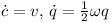
Each rigid body has a center with the 3D position c. The orientation of the object can be described using a quaternion q which has four components. The speed of the object is a 3D vector v. Finally the 3D vector ω specifies the current rotational speed of the rigid body.

The time derivatives (indicated by a dot on top of the variable name) of the position and the orientation are (Sauer et al.): The multiplication is a quaternion multiplication where the rotational speed ω is converted to a quaternion:

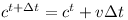
In a given time step Δt the position changes as follows

The orientation q changes as shown below Note that ω again is converted to a quaternion.

Given the mass m and the sum of external forces F the speed changes like this 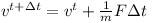In other words this means

Finally given the rotated inertia matrix I(t) and the overall torque τ one can determine the change of rotational speed Or written as a differential equation

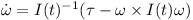
These are the Newton-Euler equations. The “x” is the vector cross product. Note that even if the overall torque τ is zero, the rotation vector still can change over time if the inertial matrix I has different eigenvalues.

The rotated inertia matrix is obtained by converting the quaternion q to a rotation matrix R and using it to rotate I₀:

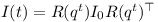
The three column vectors of R can be determined by performing quaternion rotations on the unit vectors. Note that the vectors get converted to quaternion and back implicitely.

According to David Hammen, the Newton-Euler equation can be used unmodified in the world inertial frame.

The Runge-Kutta Method

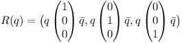
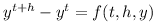
The different properties of the rigid body can be stacked in a state vector y as follows. The equations above then can be brought into the following form Using h=Δt the numerical integration for a time step can be performed using the Runge-Kutta method:

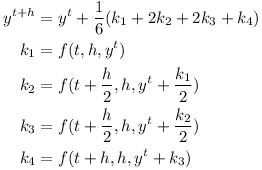
The Runge-Kutta algorithm can also be formulated using a function which instead of derivatives returns infitesimal changes

The Runge-Kutta formula then becomes

Using time-stepping with F=0 and τ=0 one can simulate an object tumbling in space.