Proximal Policy Optimization with Clojure and PyTorch

22 Apr 2026

(Cross posting article published at Clojure Civitas)

Motivation

Recently I started to look into the problem of reentry trajectory planning in the context of developing the sfsim space flight simulator. I had looked into reinforcement learning before and even tried out Q-learning using the lunar lander reference environment of OpenAI’s gym library (now maintained by the Farama Foundation). However it had stability issues. The algorithm would converge on a strategy and then suddenly diverge again.

More recently (2017) the Proximal Policy Optimization (PPO) algorithm was published and it has gained in popularity. PPO is inspired by Trust Region Policy Optimization (TRPO) but is much easier to implement. Also PPO handles continuous observation and action spaces which is important for control problems. The Stable Baselines3 Python library has a implementation of PPO, TRPO, and other reinforcement learning algorithms. However I found XinJingHao’s PPO implementation which is easier to follow.

In order to use PPO with a simulation environment implemented in Clojure and also in order to get a better understanding of PPO, I dediced to do an implementation of PPO in Clojure.

Dependencies

For this project we are using the following deps.edn file. The Python setup is shown further down in this article.

{:deps
 {org.clojure/clojure {:mvn/version "1.12.4"}
  clj-python/libpython-clj {:mvn/version "2.026"}
  quil/quil {:mvn/version "4.3.1563"}
  org.clojure/core.async {:mvn/version "1.9.865"}}
}

The dependencies can be pulled in using the following statement.

(require '[clojure.math :refer (PI cos sin exp to-radians)]
         '[clojure.core.async :as async]
         '[tablecloth.api :as tc]
         '[scicloj.tableplot.v1.plotly :as plotly]
         '[quil.core :as q]
         '[quil.middleware :as m]
         '[libpython-clj2.require :refer (require-python)]
         '[libpython-clj2.python :refer (py.) :as py])

Pendulum Environment

screenshot of pendulum environment

To validate the implementation, we will implement the classical pendulum environment in Clojure. In order to be able to switch environments, we define a protocol according to the environment abstract class used in OpenAI’s gym.

(defprotocol Environment
  (environment-update [this action])
  (environment-observation [this])
  (environment-done? [this])
  (environment-truncate? [this])
  (environment-reward [this action]))

Here is a configuration for testing the pendulum.

(def frame-rate 20)

(def config
  {:length  (/ 2.0 3.0)
   :max-speed 8.0
   :motor 6.0
   :gravitation 10.0
   :dt (/ 1.0 frame-rate)
   :save false
   :timeout 10.0
   :angle-weight 1.0
   :velocity-weight 0.1
   :control-weight 0.0001})

Setup

A method to initialise the pendulum is defined.

(defn setup
  "Initialise pendulum"
  [angle velocity]
  {:angle          angle
   :velocity       velocity
   :t              0.0})

Same as in OpenAI’s gym the angle is zero when the pendulum is pointing up. Here a pendulum is initialised to be pointing down and have an angular velocity of 0.5 radians per second.

(setup PI 0.5)
; {:angle 3.141592653589793, :velocity 0.5, :t 0.0}

State Updates

The angular acceleration due to gravitation is implemented as follows.

(defn pendulum-gravity
  "Determine angular acceleration due to gravity"
  [gravitation length angle]
  (/ (* (sin angle) gravitation) length))

The angular acceleration depends on the gravitation, length of pendulum, and angle of pendulum.

(pendulum-gravity 9.81 1.0 0.0)
; 0.0
(pendulum-gravity 9.81 1.0 (/ PI 2))
; 9.81
(pendulum-gravity 9.81 2.0 (/ PI 2))
; 4.905

The motor is controlled using an input value between -1 and 1. This value is simply multiplied with the maximum angular acceleration provided by the motor.

(defn motor-acceleration
  "Angular acceleration from motor"
  [control motor-acceleration]
  (* control motor-acceleration))

A simulation step of the pendulum is implemented using Euler integration.

(defn update-state
  "Perform simulation step of pendulum"
  ([{:keys [angle velocity t]}
    {:keys [control]}
    {:keys [dt motor gravitation length max-speed]}]
   (let [gravity        (pendulum-gravity gravitation length angle)
         motor          (motor-acceleration control motor)
         t              (+ t dt)
         acceleration   (+ motor gravity)
         velocity       (max (- max-speed)
                             (min max-speed
                                  (+ velocity (* acceleration dt))))
         angle          (+ angle (* velocity dt))]
     {:angle          angle
      :velocity       velocity
      :t              t})))

Here are a few examples for advancing the state in different situations.

(update-state {:angle PI :velocity 0.0 :t 0.0} {:control 0.0} config)
; {:angle 3.141592653589793, :velocity 9.184850993605151E-17, :t 0.05}
(update-state {:angle PI :velocity 0.1 :t 0.0} {:control 0.0} config)
; {:angle 3.146592653589793, :velocity 0.1000000000000001, :t 0.05}
(update-state {:angle (/ PI 2) :velocity 0.0 :t 0.0} {:control 0.0} config)
; {:angle 1.6082963267948966, :velocity 0.75, :t 0.05}
(update-state {:angle 0.0 :velocity 0.0 :t 0.0} {:control 1.0} config)
; {:angle 0.015000000000000003, :velocity 0.30000000000000004, :t 0.05}

Observation

The observation of the pendulum state uses cosinus and sinus of the angle to resolve the wrap around problem of angles. The angular speed is normalized to be between -1 and 1 as well. This so called feature scaling is done in order to improve convergence.

(defn observation
  "Get observation from state"
  [{:keys [angle velocity]} {:keys [max-speed]}]
  [(cos angle) (sin angle) (/ velocity max-speed)])

The observation of the pendulum is a vector with 3 elements.

(observation {:angle 0.0 :velocity 0.0} config)
; [1.0 0.0 0.0]
(observation {:angle 0.0 :velocity 0.5} config)
; [1.0 0.0 0.0625]
(observation {:angle (/ PI 2) :velocity 0.0} config)
; [6.123233995736766E-17 1.0 0.0]

Note that the observation needs to capture all information required for achieving the objective, because it is the only information available to the actor for deciding on the next action.

Action

The action of a pendulum is a vector with one element between 0 and 1. The following method clips it and converts it to an action hashmap used by the pendulum environment. Note that an action can consist of several values.

(defn action
  "Convert array to action"
  [array]
  {:control (max -1.0 (min 1.0 (- (* 2.0 (first array)) 1.0)))})

The following examples show how the action vector is mapped to a control input between -1 and 1.

(action [0.0])
; {:control -1.0}
(action [0.5])
; {:control 0.0}
(action [1.0])
; {:control 1.0}

Termination

The truncate method is used to stop a pendulum run after a specific amount of time.

(defn truncate?
  "Decide whether a run should be aborted"
  ([{:keys [t]} {:keys [timeout]}]
   (>= t timeout)))

(truncate? {:t 50.0} {:timeout 100.0})
; false
(truncate? {:t 100.0} {:timeout 100.0})
; true

It is also possible to define a termination condition. For the pendulum environment we specify that it never terminates.

(defn done?
  "Decide whether pendulum achieved target state"
  ([_state _config]
   false))

Reward

The following method normalizes an angle to be between -PI and +PI.

(defn normalize-angle
  "Angular deviation from up angle"
  [angle]
  (- (mod (+ angle PI) (* 2 PI)) PI))

We also need the square of a number.

(defn sqr
  "Square of number"
  [x]
  (* x x))

The reward function penalises deviation from the upright position, non-zero velocities, and non-zero control input. Note that it is important that the reward function is continuous because machine learning uses gradient descent.

(defn reward
  "Reward function"
  [{:keys [angle velocity]}
   {:keys [angle-weight velocity-weight control-weight]}
   {:keys [control]}]
  (- (+ (* angle-weight (sqr (normalize-angle angle)))
        (* velocity-weight (sqr velocity))
        (* control-weight (sqr control)))))

Environment Protocol

Finally we are able to implement the pendulum as a generic environment.

(defrecord Pendulum [config state]
  Environment
  (environment-update [_this input]
    (->Pendulum config (update-state state (action input) config)))
  (environment-observation [_this]
    (observation state config))
  (environment-done? [_this]
    (done? state config))
  (environment-truncate? [_this]
    (truncate? state config))
  (environment-reward [_this input]
    (reward state config (action input))))

The following factory method creates an environment with an initial random state covering all possible pendulum states.

(defn pendulum-factory
  []
  (let [angle     (- (rand (* 2.0 PI)) PI)
        max-speed (:max-speed config)
        velocity  (- (rand (* 2.0 max-speed)) max-speed)]
    (->Pendulum config (setup angle velocity))))

Visualisation

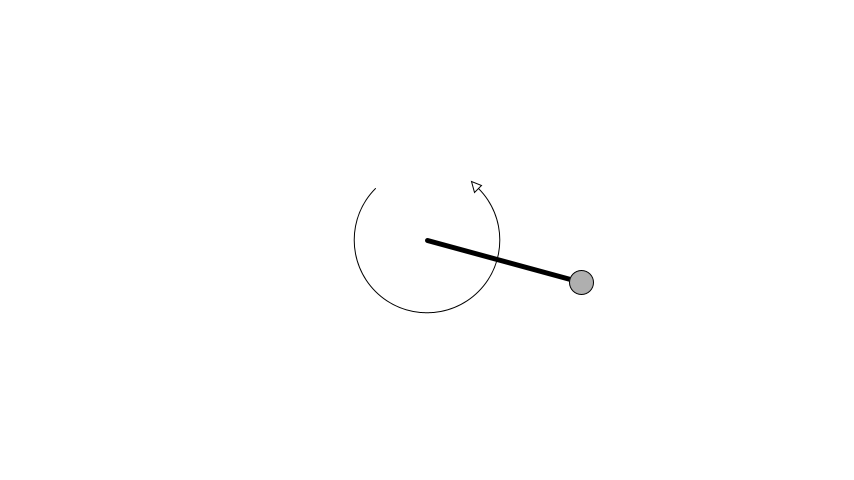
The following method is used to draw the pendulum and visualise the motor control input.

(defn draw-state [{:keys [angle]} {:keys [control]}]
  (let [origin-x   (/ (q/width) 2)
        origin-y   (/ (q/height) 2)
        length     (* 0.5 (q/height) (:length config))
        pendulum-x (+ origin-x (* length (sin angle)))
        pendulum-y (- origin-y (* length (cos angle)))
        size       (* 0.05 (q/height))
        arc-radius (* (abs control) 0.2 (q/height))
        positive   (pos? control)
        tip-angle  (if positive 225 -45)]
    (q/frame-rate frame-rate)
    (q/background 255)
    (q/stroke-weight 5)
    (q/stroke 0)
    (q/fill 175)
    (q/line origin-x origin-y pendulum-x pendulum-y)
    (q/stroke-weight 1)
    (q/ellipse pendulum-x pendulum-y size size)
    (q/no-fill)
    (q/arc origin-x origin-y
           (* 2 arc-radius) (* 2 arc-radius)
           (to-radians -45) (to-radians 225))
    (q/with-translation [(+ origin-x (* (cos (to-radians tip-angle)) arc-radius))
                         (+ origin-y (* (sin (to-radians tip-angle)) arc-radius))]
      (q/with-rotation [(to-radians (if positive 225 -45))]
        (q/triangle 0 (if positive 10 -10) -5 0 5 0)))
    (when (:save config)
      (q/save-frame "frame-####.png"))))

Animation

With Quil we can create an animation of the pendulum and react to mouse input.

(defn -main [& _args]
  (let [done-chan   (async/chan)
        last-action (atom {:control 0.0})]
    (q/sketch
      :title "Inverted Pendulum with Mouse Control"
      :size [854 480]
      :setup #(setup PI 0.0)
      :update (fn [state]
                  (let [action {:control (min 1.0
                                              (max -1.0
                                                   (- 1.0 (/ (q/mouse-x)
                                                             (/ (q/width) 2.0)))))}
                        state  (update-state state action config)]
                    (when (done? state config) (async/close! done-chan))
                    (reset! last-action action)
                    state))
      :draw #(draw-state % @last-action)
      :middleware [m/fun-mode]
      :on-close (fn [& _] (async/close! done-chan)))
    (async/<!! done-chan))
  (System/exit 0))

manually controlled pendulum

Neural Networks

PPO is a machine learning technique using backpropagation to learn the parameters of two neural networks.

The actor network takes an observation as an input and outputs the parameters of a probability distribution for sampling the next action to take.
The critic takes an observation as an input and outputs the expected cumulative reward for the current state.

Import PyTorch

For implementing the neural networks and backpropagation, we can use the Python-Clojure bridge libpython-clj2 and the PyTorch machine learning library. The PyTorch library is quite comprehensive, is free software, and you can find a lot of documentation on how to use it. The default version of PyTorch on pypi.org comes with CUDA (Nvidia) GPU support. There are also PyTorch wheels provided by AMD which come with ROCm support. Here we are going to use a CPU version of PyTorch which is a much smaller install.

You need to install Python 3.10 or later. For package management we are going to use the uv package manager. The following pyproject.toml file is used to install PyTorch and NumPy.

[project]
name = "ppo"
version = "0.1.0"
description = "Proximal Policy Optimization"
authors = [{ name="Jan Wedekind", email="jan@wedesoft.de" }]
requires-python = ">=3.10.0"
dependencies = [
    "numpy",
    "torch",
]

[tool.uv]
python-preference = "only-system"

[tool.uv.sources]
torch = { index = "pytorch" }
numpy = { index = "pytorch" }

[[tool.uv.index]]
name = "pytorch"
url = "https://download.pytorch.org/whl/cpu"

[build-system]
requires = ["setuptools", "wheel"]
build-backend = "setuptools.build_meta"

Note that we are specifying a custom repository index to get the CPU-only version of PyTorch. Also we are using the system version of Python to prevent uv from trying to install its own version which lacks the _cython module. To freeze the dependencies and create a uv.lock file, you need to run

uv lock

You can install the dependencies using

uv sync

In order to access PyTorch from Clojure you need to run the clj command via uv:

uv run clj

Now you should be able to import the Python modules using require-python.

(require-python '[builtins :as python]
                '[torch :as torch]
                '[torch.nn :as nn]
                '[torch.nn.functional :as F]
                '[torch.optim :as optim]
                '[torch.distributions :refer (Beta)]
                '[torch.nn.utils :as utils])
; :ok

Tensor Conversion

First we implement a few methods for converting nested Clojure vectors to PyTorch tensors and back.

Clojure to PyTorch

The method tensor is for converting a Clojure datatype to a PyTorch tensor.

(defn tensor
  "Convert nested vector to tensor"
  ([data]
   (tensor data torch/float32))
  ([data dtype]
   (torch/tensor data :dtype dtype)))

(tensor PI)
; tensor(3.1416)
(tensor [2.0 3.0 5.0])
; tensor([2., 3., 5.])
(tensor [[1.0 2.0] [3.0 4.0] [5.0 6.0]])
; tensor([[1., 2.],
;         [3., 4.],
;         [5., 6.]])
(tensor [1 2 3] torch/long)
; tensor([1, 2, 3])

PyTorch to Clojure

The next method is for converting a PyTorch tensor back to a Clojure datatype.

(defn tolist
  "Convert tensor to nested vector"
  [tensor]
  (py/->jvm (py. tensor tolist)))

(tolist (tensor [2.0 3.0 5.0]))
; [2.0 3.0 5.0]
(tolist (tensor [[1.0 2.0] [3.0 4.0] [5.0 6.0]]))
; [[1.0 2.0] [3.0 4.0] [5.0 6.0]]

PyTorch scalar to Clojure

A tensor with no dimensions can also be converted using toitem

(defn toitem
  "Convert torch scalar value to float"
  [tensor]
  (py. tensor item))

(toitem (tensor PI))
; 3.1415927410125732

Critic Network

The critic network is a neural network with an input layer of size observation-size and two fully connected hidden layers of size hidden-units with tanh activation functions. The critic output is a single value (an estimate for the expected cumulative return achievable by the given observed state).

(def Critic
  (py/create-class
    "Critic" [nn/Module]
    {"__init__"
     (py/make-instance-fn
       (fn [self observation-size hidden-units]
           (py. nn/Module __init__ self)
           (py/set-attrs!
             self
             {"fc1" (nn/Linear observation-size hidden-units)
              "fc2" (nn/Linear hidden-units hidden-units)
              "fc3" (nn/Linear hidden-units 1)})
           nil))
     "forward"
     (py/make-instance-fn
       (fn [self x]
           (let [x (py. self fc1 x)
                 x (torch/tanh x)
                 x (py. self fc2 x)
                 x (torch/tanh x)
                 x (py. self fc3 x)]
             (torch/squeeze x -1))))}))

When running inference, you need to run the network with gradient accumulation disabled, otherwise gradients get accumulated and can leak into a subsequent training step. In Python this looks like this.

with torch.no_grad():
    # ...

Here we create a Clojure macro to do the same job.

(defmacro without-gradient
  "Execute body without gradient calculation"
  [& body]
  `(let [no-grad# (torch/no_grad)]
     (try
       (py. no-grad# ~'__enter__)
       ~@body
       (finally
         (py. no-grad# ~'__exit__ nil nil nil)))))

Now we can create a network and try it out. We create a test multilayer perceptron with three inputs, two hidden layers of 8 units each, and one output.

(def critic (Critic 3 8))

example of critic multilayer perceptron

Note that the network creates non-zero outputs because PyTorch performs random initialisation of the weights for us.

(without-gradient
  (toitem (critic (tensor [-1 0 0]))))
; -0.38925105333328247

We can also create a wrapper for using the neural network with Clojure datatypes.

(defn critic-observation
  "Use critic with Clojure datatypes"
  [critic]
  (fn [observation]
      (without-gradient (toitem (critic (tensor observation))))))

Here is the output of the network for the observation [-1 0 0].

((critic-observation critic) [-1 0 0])
; -0.38925105333328247

Training

Training a neural network is done by defining a loss function. The loss of the network then is calculated for a mini-batch of training data. One can then use PyTorch’s backpropagation to compute the gradient of the loss value with respect to every single parameter of the network. The gradient then is used to perform a gradient descent step. A popular gradient descent method is the Adam optimizer.

Here is a wrapper for the Adam optimizer.

(defn adam-optimizer
  "Adam optimizer"
  [model learning-rate weight-decay]
  (optim/Adam (py. model parameters) :lr learning-rate :weight_decay weight-decay))

PyTorch also provides the mean square error (MSE) loss function.

(defn mse-loss
  "Mean square error cost function"
  []
  (nn/MSELoss))

A training step can be performed as follows. Here we only use a single mini-batch with a single observation and an expected output of 1.0.

(def optimizer (adam-optimizer critic 0.01 0.0))
(def criterion (mse-loss))
(def mini-batch [(tensor [[-1 0 0]]) (tensor [1.0])])
(let [prediction (critic (first mini-batch))
      expected   (second mini-batch)
      loss       (criterion prediction expected)]
  (py. optimizer zero_grad)
  (py. loss backward)
  (py. optimizer step))

As you can see, the output of the network for the observation [-1 0 0] is now closer to 1.0.

((critic-observation critic) [-1 0 0])
; -0.3086397051811218

Actor Network

The actor network for PPO takes an observation as an input and it outputs the parameters of a probability distribution over actions. In addition to the forward pass, the actor network has a method deterministic_act to choose the expectation value of the distribution as a deterministic action.

(def Actor
  (py/create-class
    "Actor" [nn/Module]
    {"__init__"
     (py/make-instance-fn
       (fn [self observation-size hidden-units action-size]
           (py. nn/Module __init__ self)
           (py/set-attrs!
             self
             {"fc1"     (nn/Linear observation-size hidden-units)
              "fc2"     (nn/Linear hidden-units hidden-units)
              "fcalpha" (nn/Linear hidden-units action-size)
              "fcbeta"  (nn/Linear hidden-units action-size)})
           nil))
     "forward"
     (py/make-instance-fn
       (fn [self x]
           (let [x (py. self fc1 x)
                 x (torch/tanh x)
                 x (py. self fc2 x)
                 x (torch/tanh x)
                 alpha (torch/add 1.0 (F/softplus (py. self fcalpha x)))
                 beta  (torch/add 1.0 (F/softplus (py. self fcbeta x)))]
             [alpha beta])))
     "deterministic_act"
     (py/make-instance-fn
       (fn [self x]
            (let [[alpha beta] (py. self forward x)]
              (torch/div alpha (torch/add alpha beta)))))
     "get_dist"
     (py/make-instance-fn
       (fn [self x]
           (let [[alpha beta] (py. self forward x)]
             (Beta alpha beta))))}))

Furthermore the actor network has a method get_dist to return a Torch distribution object which can be used to sample a random action or query the current log-probability of an action. Here (as the default in XinJingHao’s PPO implementation) we use the Beta distribution with parameters alpha and beta both greater than 1.0. See here for an interactive visualization of the Beta distribution.

(defn indeterministic-act
  "Sample action using actor network returning random action and log-probability"
  [actor]
  (fn indeterministic-act-with-actor [observation]
      (without-gradient
        (let [dist    (py. actor get_dist (tensor observation))
              sample  (py. dist sample)
              action  (torch/clamp sample 0.0 1.0)
              logprob (py. dist log_prob action)]
          {:action (tolist action) :logprob (tolist logprob)}))))

We create a test multilayer perceptron with three inputs, two hidden layers of 8 units each, and two outputs which serve as parameters for the Beta distribution.

(def actor (Actor 3 8 1))

example of actor multilayer perceptron

One can then use the network to:

a. get the parameters of the distribution for a given observation.

(without-gradient (actor (tensor [-1 0 0])))
; (tensor([1.7002]), tensor([1.7489]))

b. choose the expectation value of the distribution as an action.

(without-gradient (py. actor deterministic_act (tensor [-1 0 0])))
; tensor([0.4929])

c. sample a random action from the distribution and get the associated log-probability.

((indeterministic-act actor) [-1 0 0])
{:action [0.6526480913162231], :logprob [0.2350209504365921]}

We can also query the current log-probability of a previously sampled action.

(defn logprob-of-action
  "Get log probability of action"
  [actor]
  (fn [observation action]
      (let [dist (py. actor get_dist observation)]
        (py. dist log_prob action))))

Here is a plot of the probability density function (PDF) actor output for a single observation.

(without-gradient
  (let [actions (range 0.0 1.01 0.01)
        logprob (fn [action]
                    (tolist
                      ((logprob-of-action actor) (tensor [-1 0 0]) (tensor action))))
        scatter (tc/dataset
                  {:x actions
                   :y (map (fn [action] (exp (first (logprob [action])))) actions)})]
    (-> scatter
        (plotly/base {:=title "Actor output for a single observation" :=mode :lines})
        (plotly/layer-point {:=x :x :=y :y}))))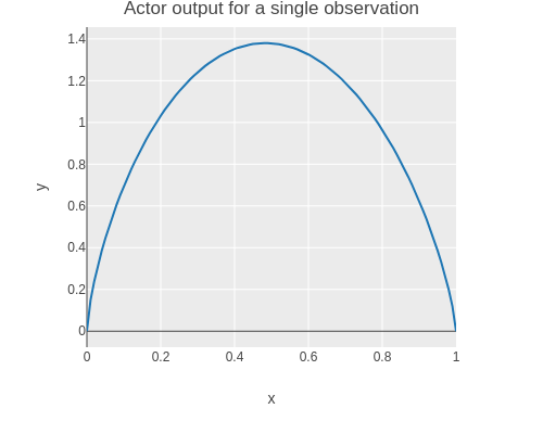

probability density function output of actor for a single observation

Finally we can also query the entropy of the distribution. By incorporating the entropy into the loss function later on, we can encourage exploration and prevent the probability density function from collapsing.

(defn entropy-of-distribution
  "Get entropy of distribution"
  [actor observation]
  (let [dist (py. actor get_dist observation)]
    (py. dist entropy)))

(without-gradient (entropy-of-distribution actor (tensor [-1 0 0])))
; tensor([-0.0825])

Proximal Policy Optimization

Sampling data

In order to perform optimization, we sample the environment using the current policy (indeterministic action using actor).

(defn sample-environment
  "Collect trajectory data from environment"
  [environment-factory policy size]
  (loop [state             (environment-factory)
         observations      []
         actions           []
         logprobs          []
         next-observations []
         rewards           []
         dones             []
         truncates         []
         i                 size]
    (if (pos? i)
      (let [observation      (environment-observation state)
            sample           (policy observation)
            action           (:action sample)
            logprob          (:logprob sample)
            reward           (environment-reward state action)
            done             (environment-done? state)
            truncate         (environment-truncate? state)
            next-state       (if (or done truncate)
                               (environment-factory)
                               (environment-update state action))
            next-observation (environment-observation next-state)]
        (recur next-state
               (conj observations observation)
               (conj actions action)
               (conj logprobs logprob)
               (conj next-observations next-observation)
               (conj rewards reward)
               (conj dones done)
               (conj truncates truncate)
               (dec i)))
      {:observations      observations
       :actions           actions
       :logprobs          logprobs
       :next-observations next-observations
       :rewards           rewards
       :dones             dones
       :truncates         truncates})))

Here for example we are sampling 3 consecutives states of the pendulum.

(sample-environment pendulum-factory (indeterministic-act actor) 3)
; {:observations
;  [[-0.7596729533565417 0.6503053159390207 0.5479034035454418]
;   [-0.8900589293843874 0.4558454806435161 0.5866609335014912]
;   [-0.9762048336009674 0.21685046196424718 0.6368372482766531]],
;  :actions
;  [[0.20388542115688324] [0.5992106795310974] [0.1662445366382599]],
;  :logprobs
;  [[0.08455279469490051] [0.26384592056274414] [-0.028919726610183716]],
;  :next-observations
;  [[-0.8900589293843874 0.4558454806435161 0.5866609335014912]
;   [-0.9762048336009674 0.21685046196424718 0.6368372482766531]
;   [-0.99941293940555 -0.034260422483655656 0.6321353193336707]],
;  :rewards [-7.8437431872499745 -9.322367484397839 -11.139601368813137],
;  :dones [false false false],
;  :truncates [false false false]}

Advantages

Theory

If we are in state \(s_t\) and take an action \(a_t\) at timestep \(t\), we receive reward \(r_t\) and end up in state \(s_{t+1}\). The cumulative reward for state \(s_t\) is a finite or infinite sequence using a discount factor \(γ<1\):

\(r_t + \gamma r_{t+1} + \gamma^2 r_{t+2} + \gamma^3 r_{t+3} + \ldots\)

The critic \(V\) estimates the expected cumulative reward for starting from the specified state.

\(V(s_t) = \mathop{\hat{\mathbb{E}}} [ r_t + \gamma r_{t+1} + \gamma^2 r_{t+2} + \gamma^3 r_{t+3} + \ldots ]\)

In particular, the difference between discounted rewards can be used to get an estimate for the individual reward:

\(V(s_t) = \mathop{\hat{\mathbb{E}}} [ r_t ] + \gamma V(s_{t+1})\Leftrightarrow\mathop{\hat{\mathbb{E}}} [ r_t ] = V(s_t) - \gamma V(s_{t+1})\)

The deviation of the individual reward received in state \(s_t\) from the expected reward is:

\(\delta_t = r_t + \gamma V(s_{t+1}) - V(s_t)\mathrm{\ if\ not\ }\operatorname{done}_t\)

The special case where a time series is “done” (and the next one is started) uses 0 as the remaining expected cumulative reward.

\(\delta_t = r_t - V(s_t)\mathrm{\ if\ }\operatorname{done}_{t}\)

If we have a sample set with a sequence of \(T\) states (\(t=0,1,\ldots,T-1\)), one can compute the cumulative advantage for each time step going backwards:

\(\hat{A} _ {T-1} = -V(s_{T-1}) + r_{T-1} + \gamma V(s_T) = \delta_{T-1}\)

\(\hat{A} _ {T-2} = -V(s_{T-2}) + r_{T-2} + \gamma r_{T-1} + \gamma^2 V(s_T) = \delta_{T-2} + \gamma \delta_{T-1}\)

\(\vdots\)

\(\hat{A} _ 0 = -V(s_0) + r_0 + \gamma r_1 + \gamma^2 r_2 + \ldots + + \gamma^{T-1} r_{T-1} + \gamma^{T} V(s_{T})\)

\(\hphantom{\hat{A} _ 0} = \delta_0 + \gamma \delta_1 + \gamma^2 \delta_2 + \ldots + \gamma^{T-1} \delta_{T-1}\)

I.e. we can compute the cumulative advantages as follows:

Start with \(\hat{A} _ {T-1} = \delta_{T-1}\)
Continue with \(\hat{A} _ t = \delta_t + \gamma \hat{A} _ {t+1}\) for \(t=T-2,T-3,\ldots,0\)

PPO uses an additional factor λ≤1 called Generalized Advantage Estimation (GAE) which can be used to steer the training towards more immediate rewards if there are stability issues. See Schulman et al. for more details.

Implementation of Deltas

The code for computing the \(\delta\) values follows here:

(defn deltas
  "Compute difference between actual reward plus discounted estimate of next state and estimated value of current state"
  [{:keys [observations next-observations rewards dones]} critic gamma]
  (mapv (fn [observation next-observation reward done]
            (- (+ reward
                  (if done 0.0 (* gamma (critic next-observation))))
               (critic observation)))
        observations next-observations rewards dones))

If the reward is zero and the critic outputs constant zero, there is no difference between the expected and received reward.

(deltas {:observations [[4]] :next-observations [[3]] :rewards [0] :dones [false]}
        (constantly 0)
        1.0)
; [0.0]

If the reward is 1.0 and the critic outputs zero for both observations, the difference is 1.0.

(deltas {:observations [[4]] :next-observations [[3]] :rewards [1] :dones [false]}
        (constantly 0)
        1.0)
; [1.0]

If the reward is 1.0 and the difference of critic outputs is also 1.0 then there is no difference between the expected and received reward (when \(\gamma=1\)).

(defn linear-critic [observation] (first observation))
(deltas {:observations [[4]] :next-observations [[3]] :rewards [1] :dones [false]}
        linear-critic
        1.0)
; [0.0]

If the next critic value is 1.0 and discounted with 0.5 and the current critic value is 2.0, we expect a reward of 1.5. If we only get a reward of 1.0, the difference is -0.5.

(deltas {:observations [[2]] :next-observations [[1]] :rewards [1] :dones [false]}
        linear-critic
        0.5)
; [-0.5]

If the run is terminated, the current critic value is compared with the reward which in this case is the last reward received in this run.

(deltas {:observations [[4]] :next-observations [[3]] :rewards [4] :dones [true]}
        linear-critic
        1.0)
; [0.0]

Implementation of Advantages

The advantages can be computed in an elegant way using reductions and the previously computed deltas.

(defn advantages
  "Compute advantages attributed to each action"
  [{:keys [dones truncates]} deltas gamma lambda]
  (vec
    (reverse
    (rest
      (reductions
        (fn [advantage [delta done truncate]]
            (+ delta (if (or done truncate) 0.0 (* gamma lambda advantage))))
        0.0
        (reverse (map vector deltas dones truncates)))))))

For example when all deltas are 1.0 and if using an discount factor of 0.5, the advantages approach 2.0 assymptotically when going backwards in time.

(advantages {:dones [false false false] :truncates [false false false]}
            [1.0 1.0 1.0]
            0.5
            1.0)
; [1.75 1.5 1.0]

When an episode is terminated (or truncated), the accumulation of advantages starts again when going backwards in time. I.e. the computation of advantages does not distinguish between terminated and truncated episodes (unlike the deltas).

(advantages {:dones [false false true false false true]
             :truncates [false false false false false false]}
            [1.0 1.0 1.0 1.0 1.0 1.0]
            0.5
            1.0)
; [1.75 1.5 1.0 1.75 1.5 1.0]

We add the advantages to the batch of samples with the following function.

(defn assoc-advantages
  "Associate advantages with batch of samples"
  [critic gamma lambda batch]
  (let [deltas     (deltas batch critic gamma)
        advantages (advantages batch deltas gamma lambda)]
    (assoc batch :advantages advantages)))

Critic Loss Function

The target values for the critic are simply the current values plus the new advantages. The target values can be computed using PyTorch’s add function.

(defn critic-target
  "Determine target values for critic"
  [{:keys [observations advantages]} critic]
  (without-gradient (torch/add (critic observations) advantages)))

We add the critic targets to the batch of samples with the following function.

(defn assoc-critic-target
  "Associate critic target values with batch of samples"
  [critic batch]
  (let [target (critic-target batch critic)]
    (assoc batch :critic-target target)))

If we add the target values to the samples, we can compute the critic loss for a batch of samples as follows.

(defn critic-loss
  "Compute loss value for batch of samples and critic"
  [samples critic]
  (let [criterion (mse-loss)
        loss      (criterion (critic (:observations samples)) (:critic-target samples))]
    loss))

Actor Loss Function

The core of the actor loss function relies on the action probability ratio of using the updated and the old policy (actor network output). The ratio is defined as \(r_t(\theta)=\frac{\pi_\theta(a_t|s_t)}{\pi_{\theta_{\operatorname{old}}}(a_t|s_t)}\).

Note that \(r_t(\theta)\) here refers to the probability ratio as opposed to the reward of the previous section.

The sampled observations, log probabilities, and actions are combined with the actor’s parameter-dependent log probabilities.

(defn probability-ratios
  "Probability ratios for a actions using updated policy and old policy"
  [{:keys [observations logprobs actions]} logprob-of-action]
  (let [updated-logprobs (logprob-of-action observations actions)]
    (torch/exp (py. (torch/sub updated-logprobs logprobs) sum 1))))

The objective is to increase the probability of actions which lead to a positive advantage and reduce the probability of actions which lead to a negative advantage. I.e. maximising the following objective function.

\(L^{CPI}(\theta) = \mathop{\hat{\mathbb{E}}}_t [\frac{\pi _ \theta(a_t|s_t)}{\pi _ {\theta _ {\operatorname{old}}} (a_t|s_t)} \hat{A}_t] = \mathop{\hat{\mathbb{E}}}_t [r_t (\theta) \hat{A}_t]\)

The core idea of PPO is to use clipped probability ratios for the loss function in order to increase stability, . The probability ratio is clipped to stay below 1+ε for positive advantages and to stay above 1-ε for negative advantages.

\(L^{CLIP}(\theta) = \mathop{\hat{\mathbb{E}}}_t [\min(r_t (\theta) \hat{A}_t, \mathop{\operatorname{clip}}(r_t (\theta), 1-\epsilon, 1+\epsilon) \hat{A}_t)]\)

See Schulman et al. for more details.

Because PyTorch minimizes a loss, we need to negate above objective function.

(defn clipped-surrogate-loss
  "Clipped surrogate loss (negative objective)"
  [probability-ratios advantages epsilon]
  (torch/mean
    (torch/neg
      (torch/min
        (torch/mul probability-ratios advantages)
        (torch/mul (torch/clamp probability-ratios (- 1.0 epsilon) (+ 1.0 epsilon))
                   advantages)))))

We can plot the objective function for a single action and a positive advantage.

(without-gradient
  (let [ratios  (range 0.0 2.01 0.01)
        loss    (fn [ratio advantage epsilon]
                    (toitem
                      (torch/neg
                        (clipped-surrogate-loss (tensor ratio)
                                                (tensor advantage)
                                                epsilon))))
        scatter (tc/dataset
                  {:x ratios
                   :y (map (fn [ratio] (loss ratio 0.5 0.2)) ratios)})]
    (-> scatter
        (plotly/base {:=title "Objective Function for Positive Advantage" :=mode :lines})
        (plotly/layer-point {:=x :x :=y :y}))))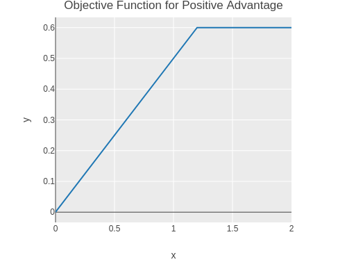

actor loss over ratio for positive advantage

And for a negative advantage.

(without-gradient
  (let [ratios  (range 0.0 2.01 0.01)
        loss    (fn [ratio advantage epsilon]
                    (toitem
                      (torch/neg
                        (clipped-surrogate-loss (tensor ratio)
                                                (tensor advantage)
                                                epsilon))))
        scatter (tc/dataset
                  {:x ratios
                   :y (map (fn [ratio] (loss ratio -0.5 0.2)) ratios)})]
    (-> scatter
        (plotly/base {:=title "Objective Function for Negative Advantage" :=mode :lines})
        (plotly/layer-point {:=x :x :=y :y}))))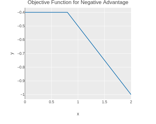

actor loss over ratio for positive advantage

We can now implement the actor loss function which we want to minimize. The loss function uses the clipped surrogate loss function as defined above. The loss function also penalises low entropy values of the distributions output by the actor in order to encourage exploration.

(defn actor-loss
  "Compute loss value for batch of samples and actor"
  [samples actor epsilon entropy-factor]
  (let [ratios         (probability-ratios samples (logprob-of-action actor))
        entropy        (torch/mul
                         entropy-factor
                         (torch/neg
                           (torch/mean
                             (entropy-of-distribution actor (:observations samples)))))
        surrogate-loss (clipped-surrogate-loss ratios (:advantages samples) epsilon)]
    (torch/add surrogate-loss entropy)))

A notable detail in XinJingHao’s PPO implementation is that the advantage values used in the actor loss (not in the critic loss!) are normalized.

(defn normalize-advantages
  "Normalize advantages"
  [batch]
  (let [advantages (:advantages batch)]
    (assoc batch :advantages (torch/div (torch/sub advantages (torch/mean advantages))
                                        (torch/std advantages)))))

Preparing Samples

Shuffling

The data required for training needs to be converted to PyTorch tensors.

(defn tensor-batch
  "Convert batch to Torch tensors"
  [batch]
  {:observations (tensor (:observations batch))
   :logprobs (tensor (:logprobs batch))
   :actions (tensor (:actions batch))
   :advantages (tensor (:advantages batch))})

Furthermore it is good practice to shuffle the samples. This ensures that samples early and late in the sequence are not threated differently. Note that you need to shuffle after computing the advantages, because the computation of the advantages relies on the order of the samples.

We separate the generation of random indices to facilitate unit testing of the shuffling function.

(defn random-order
  "Create a list of randomly ordered indices"
  [n]
  (shuffle (range n)))

(defn shuffle-samples
  "Random shuffle of samples"
  ([samples]
   (shuffle-samples samples (random-order (python/len (first (vals samples))))))
  ([samples indices]
   (zipmap (keys samples)
           (map #(torch/index_select % 0 (torch/tensor indices)) (vals samples)))))

Here is an example of shuffling observations:

(shuffle-samples {:observations (tensor [[1] [2] [3] [4] [5] [6] [7] [8] [9] [10]])})
; {:observations tensor([[ 1.],
;         [ 4.],
;         [ 6.],
;         [ 5.],
;         [10.],
;         [ 8.],
;         [ 7.],
;         [ 2.],
;         [ 9.],
;         [ 3.]])}

Creating Batches

Furthermore we split up the samples into smaller batches to improve training speed.

(defn create-batches
  "Create mini batches from environment samples"
  [batch-size samples]
  (apply mapv
         (fn [& args] (zipmap (keys samples) args))
         (map #(py. % split batch-size) (vals samples))))

(create-batches 5 {:observations (tensor [[1] [2] [3] [4] [5] [6] [7] [8] [9] [10]])})
; [{:observations tensor([[1.],
;         [2.],
;         [3.],
;         [4.],
;         [5.]])} {:observations tensor([[ 6.],
;         [ 7.],
;         [ 8.],
;         [ 9.],
;         [10.]])}]

Putting it All Together

Finally we can implement a method which

samples data
adds advantages
converts to PyTorch tensors
adds critic targets
normalizes the advantages
shuffles the samples
creates batches

(defn sample-with-advantage-and-critic-target
  "Create batches of samples and add add advantages and critic target values"
  [environment-factory actor critic size batch-size gamma lambda]
  (->> (sample-environment environment-factory (indeterministic-act actor) size)
       (assoc-advantages (critic-observation critic) gamma lambda)
       tensor-batch
       (assoc-critic-target critic)
       normalize-advantages
       shuffle-samples
       (create-batches batch-size)))

PPO Main Loop

Now we can implement the PPO main loop.

The outer loop samples the environment using the current actor (i.e. policy) and computes the data required for training.

The inner loop performs a small number of updates using the samples from the outer loop.

Each update step performs a gradient descent update for the actor and a gradient descent update for the critic. Another detail from XinJingHao’s PPO implementation is that the gradient norm for the actor update is clipped.

At the end of the loop, the smoothed loss values are shown and the deterministic actions and entropies for a few observations are shown which helps with parameter tuning. Furthermore the entropy factor is slowly lowered so that the policy reduces exploration over time.

The actor and critic model are saved to disk after each checkpoint.

(defn -main [& _args]
  (let [factory          pendulum-factory
        actor            (Actor 3 64 1)
        critic           (Critic 3 64)
        n-epochs         100000
        n-updates        10
        gamma            0.99
        lambda           1.0
        epsilon          0.2
        n-batches        8
        batch-size       50
        checkpoint       100
        entropy-factor   (atom 0.1)
        entropy-decay    0.999
        lr               5e-5
        weight-decay     1e-4
        smooth-actor-loss  (atom 0.0)
        smooth-critic-loss (atom 0.0)
        actor-optimizer  (adam-optimizer actor lr weight-decay)
        critic-optimizer (adam-optimizer critic lr weight-decay)]
    (doseq [epoch (range n-epochs)]
           (let [samples (sample-with-advantage-and-critic-target factory actor critic
                                                                  (* batch-size n-batches)
                                                                  batch-size
                                                                  gamma lambda)]
             (doseq [k (range n-updates)]
                    (doseq [batch samples]
                           (let [loss (actor-loss batch actor epsilon @entropy-factor)]
                             (py. actor-optimizer zero_grad)
                             (py. loss backward)
                             (utils/clip_grad_norm_(py. actor parameters) 0.5)
                             (py. actor-optimizer step)
                             (swap! smooth-actor-loss
                                    (fn [x] (+ (* 0.999 x) (* 0.001 (toitem loss))))) ))
                    (doseq [batch samples]
                           (let [loss (critic-loss batch critic)]
                             (py. critic-optimizer zero_grad)
                             (py. loss backward)
                             (py. critic-optimizer step)
                             (swap! smooth-critic-loss
                                    (fn [x] (+ (* 0.999 x) (* 0.001 (toitem loss))))))))
             (println "Epoch:" epoch
                      "Actor Loss:" @smooth-actor-loss
                      "Critic Loss:" @smooth-critic-loss
                      "Entropy Factor:" @entropy-factor))
           (without-gradient
             (doseq [input [[1 0 -1.0] [1 0 1.0] [0 -1 -1.0] [0 -1 1.0] [0 1 -1.0] [0 1 1.0] [-1 0 -1.0] [-1 0 1.0]]]
                    (println
                      input
                      "->" (action (tolist (py. actor deterministic_act (tensor input))))
                      "entropy" (toitem (entropy-of-distribution actor (tensor input))))))
           (swap! entropy-factor * entropy-decay)
           (when (= (mod epoch checkpoint) (dec checkpoint))
             (println "Saving models")
             (torch/save (py. actor state_dict) "actor.pt")
             (torch/save (py. critic state_dict) "critic.pt")))
    (torch/save (py. actor state_dict) "actor.pt")
    (torch/save (py. critic state_dict) "critic.pt")
    (System/exit 0)))

Visualisation of Actor Output

We can use dtype-next to visualise the output of the actor. First we need to load additional modules.

(require '[tech.v3.datatype :as dtype]
         '[tech.v3.tensor :as dtt]
         '[tech.v3.libs.buffered-image :as bufimg]
         '[tech.v3.datatype.functional :as dfn])

Here we load a pre-trained model and visualise the output of the actor.

(def actor (Actor 3 64 1))
(py. actor load_state_dict (torch/load "src/ppo/actor.pt"))
; <All keys matched successfully>

(let [angle-values   (torch/linspace (- PI) PI 854)
      speed-values   (torch/linspace 1.0 -1.0 480)
      grid           (torch/meshgrid speed-values angle-values :indexing "ij")
      cos-angle      (torch/cos (last grid))
      sin-angle      (torch/sin (last grid))
      observations   (torch/stack [(py. cos-angle ravel)
                                   (py. sin-angle ravel)
                                   (py. (first grid) ravel)]
                                  :axis 1)
      actions        (without-gradient
                       (py. (py. (py. actor deterministic_act observations)
                                 reshape 480 854) numpy))
      actions-tensor (dtt/clone
                       (dtype/elemwise-cast (dtt/ensure-tensor (py/->jvm actions))
                                            :float32))
      actions-trsps  (dtt/transpose actions-tensor [1 0])]
  (dtt/mset! actions-tensor 240 (dfn/- 1.0 (actions-tensor 240)))
  (dtt/mset! actions-trsps 427 (dfn/- 1.0 (actions-trsps 427)))
  (bufimg/tensor->image (dfn/* actions-tensor 255)))

Actor function output over state space This image shows the motor control input as a function of pendulum angle and angular velocity. As one can see, the pendulum is decelerated when the speed is high (dark values at the top of the image). Near the centre of the image (speed zero and angle zero) one can see how the pendulum is accelerated when the angle is negative and the speed small and decelerated when the angle is positive and the speed is small. Also the image is not symmetrical because otherwise the pendulum would not start swinging up when pointing downwards (left and right boundary of the image).

Automated Pendulum

The pendulum implementation can now be updated to use the actor instead of the mouse position as motor input when the mouse button is pressed.

(defn -main [& _args]
  (let [actor       (Actor 3 64 1)
        done-chan   (async/chan)
        last-action (atom {:control 0.0})]
    (when (.exists (java.io.File. "actor.pt"))
      (py. actor load_state_dict (torch/load "actor.pt")))
    (q/sketch
      :title "Inverted Pendulum with Mouse Control"
      :size [854 480]
      :setup #(setup PI 0.0)
      :update (fn [state]
                  (let [observation (observation state config)
                        action      (if (q/mouse-pressed?)
                                      (action (tolist (py. actor
                                                           deterministic_act
                                                           (tensor observation))))
                                      {:control (min 1.0
                                                     (max -1.0
                                                          (- 1.0 (/ (q/mouse-x)
                                                                    (/ (q/width) 2.0)))))})
                        state       (update-state state action config)]
                    (when (done? state config) (async/close! done-chan))
                    (reset! last-action action)
                    state))
      :draw #(draw-state % @last-action)
      :middleware [m/fun-mode]
      :on-close (fn [& _] (async/close! done-chan)))
    (async/<!! done-chan))
  (System/exit 0))

Here is a small demo video of the pendulum being controlled using the actor network. You can find a repository with the code of this article as well as unit tests at github.com/wedesoft/ppo.

automatically controlled pendulum

Enjoy!