There is a recent article on Clojure Civitas on using Scittle for browser native slides.
Scittle is a Clojure interpreter that runs in the browser.
It even defines a script tag that let’s you embed Clojure code in your HTML code.
Here is an example evaluating the content of an HTML textarea:
The following function is used to create screenshots for this article.
We read the pixels, write them to a temporary file using the STB library and then convert it to an ImageIO object.
In the fragment shader we use the pixel coordinates to output a color ramp.
The uniform variable iResolution will later be set to the window resolution.
Note: It is beyond the topic of this talk, but you can set up a Clojure function to test an OpenGL shader function by using a probing fragment shader and rendering to a one pixel texture.
Please see my article Test Driven Development with OpenGL for more information!
Creating vertex buffer data
To provide the shader program with vertex data we are going to define just a single quad consisting of four vertices.
First we define a macro and use it to define convenience functions for converting arrays to LWJGL buffer objects.
Now we use the function to setup the VAO, VBO, and IBO.
(defvao(setup-vaoverticesindices))
The data of each vertex is defined by 3 floats (x, y, z).
We need to specify the layout of the vertex buffer object so that OpenGL knows how to interpret it.
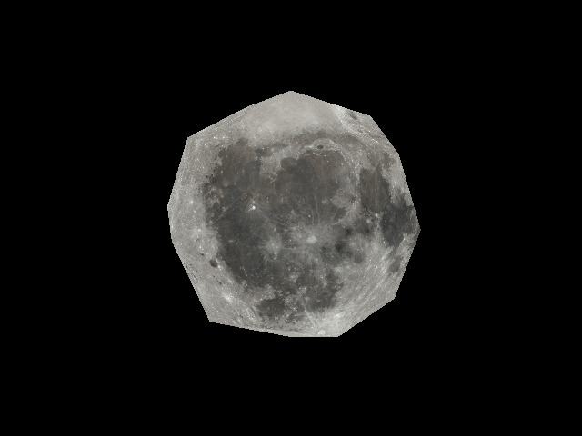
We can now use vector math to subsample the faces and project the points onto a sphere by normalizing the vectors and multiplying with the moon radius.
In order to introduce lighting we add ambient and diffuse lighting to the fragment shader.
We use the ambient and diffuse lighting from the Phong shading model.
The ambient light is a constant value.
The diffuse light is calculated using the dot product of the light vector and the normal vector.
In 2017 I discovered the free of charge Orbiter 2016 space flight simulator which was proprietary at the time and it inspired me to develop a space flight simulator myself.
I prototyped some rigid body physics in C and later in GNU Guile and also prototyped loading and rendering of Wavefront OBJ files.
I used GNU Guile (a Scheme implementation) because it has a good native interface and of course it has hygienic macros.
Eventually I got interested in Clojure because it has more generic multi-methods as well as fast hash maps and vectors.
I finally decided to develop the game for real in Clojure.
I have been developing a space flight simulator in Clojure for almost 5 years now.
While using Clojure I have come to appreciate the immutable values and safe parallelism using atoms, agents, and refs.
In the beginning I decided to work on the hard parts first, which for me were 3D rendering of a planet, an atmosphere, shadows, and volumetric clouds.
I read the OpenGL Superbible to get an understanding on what functionality OpenGL provides.
When Orbiter was eventually open sourced and released unter MIT license here, I inspected the source code and discovered that about 90% of the code is graphics-related.
So starting with the graphics problems was not a bad decision.
Software dependencies
The following software is used for development.
The software libraries run on both GNU/Linux and Microsoft Windows.
In order to manage the different dependencies for Microsoft Windows, a separate Git branch is maintained.
Atmosphere rendering
For the atmosphere, Bruneton’s precomputed atmospheric scattering was used.
The implementation uses a 2D transmittance table, a 2D surface scattering table, a 4D Rayleigh scattering, and a 4D Mie scattering table.
The tables are computed using several iterations of numerical integration.
Higher order functions for integration over a sphere and over a line segment were implemented in Clojure.
Integration over a ray in 3D space (using fastmath vectors) was implemented as follows for example:
(defnintegral-ray"Integrate given function over a ray in 3D space"{:malli/schema[:=>[:catrayN:double[:=>[:cat[:vector:double]]:some]]:some]}[{::keys[origindirection]}stepsdistancefun](let[stepsize(/distancesteps)samples(mapv#(*(+0.5%)stepsize)(rangesteps))interpolate(fninterpolate[s](addorigin(multdirections)))direction-len(magdirection)](reduceadd(mapv#(->%interpolatefun(mult(*stepsizedirection-len)))samples))))
Precomputing the atmospheric tables takes several hours even though pmap was used.
When sampling the multi-dimensional functions, pmap was used as a top-level loop and map was used for interior loops.
Using java.nio.ByteBuffer the floating point values were converted to a byte array and then written to disk using a clojure.java.io/output-stream:
(defnfloats->bytes"Convert float array to byte buffer"[^floatsfloat-data](let[n(countfloat-data)byte-buffer(.order(ByteBuffer/allocate(*n4))ByteOrder/LITTLE_ENDIAN)](.put(.asFloatBufferbyte-buffer)float-data)(.arraybyte-buffer)))(defnspit-bytes"Write bytes to a file"{:malli/schema[:=>[:catnon-empty-stringbytes?]:nil]}[^Stringfile-name^bytesbyte-data](with-open[out(io/output-streamfile-name)](.writeoutbyte-data)))(defnspit-floats"Write floating point numbers to a file"{:malli/schema[:=>[:catnon-empty-stringseqable?]:nil]}[^Stringfile-name^floatsfloat-data](spit-bytesfile-name(floats->bytesfloat-data)))
When launching the game, the lookup tables get loaded and copied into OpenGL textures.
Shader functions are used to lookup and interpolate values from the tables.
When rendering the planet surface or the space craft, the atmosphere essentially gets superimposed using ray tracing.
After rendering the planet, a background quad is rendered to display the remaining part of the atmosphere above the horizon.
Templating OpenGL shaders
It is possible to make programming with OpenGL shaders more flexible by using a templating library such as Comb.
The following shader defines multiple octaves of noise on a base noise function:
One can then for example define the function fbm_noise using octaves of the base function noise as follows:
(defnoise-octaves"Shader function to sum octaves of noise"(template/fn[method-namebase-functionoctaves](slurp"resources/shaders/core/noise-octaves.glsl"))); ...(deffbm-noise-shader(noise-octaves"fbm_noise""noise"[0.570.280.15]))
Planet rendering
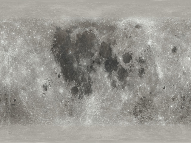
To render the planet, NASA Bluemarble data, NASA Blackmarble data, and NASA Elevation data was used.
The images were converted to a multi resolution pyramid of map tiles.
The following functions were implemented for color map tiles and for elevation tiles:
a function to load and cache map tiles of given 2D tile index and level of detail
a function to extract a pixel from a map tile
a function to extract the pixel for a specific longitude and latitude
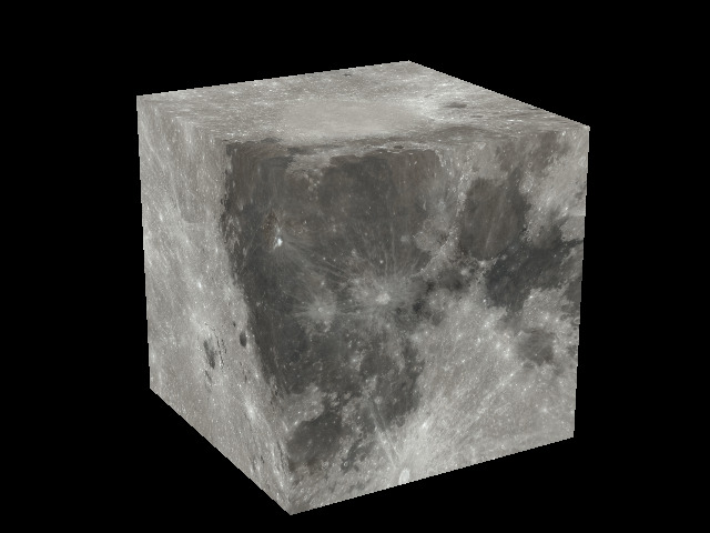
The functions for extracting a pixel for given longitude and latitude then were used to generate a cube map with a quad tree of tiles for each face.
For each tile, the following files were generated:
A daytime texture
A night time texture
An image of 3D vectors defining a surface mesh
A water mask
A normal map
Altogether 655350 files were generated.
Because the Steam ContentBuilder does not support a large number of files, each row of tile data was aggregated into a tar file.
The Apache Commons Compress library allows you to open a tar file to get a list of entries and then perform random access on the contents of the tar file.
A Clojure LRU cache was used to maintain a cache of open tar files for improved performance.
At run time, a future is created, which returns an updated tile tree, a list of tiles to drop, and a path list of the tiles to load into OpenGL.
When the future is realized, the main thread deletes the OpenGL textures from the drop list, and then uses the path list to get the new loaded images from the tile tree, load them into OpenGL textures, and create an updated tile tree with the new OpenGL textures added.
The following functions to manipulate quad trees were implemented to realize this:
(defnquadtree-add"Add tiles to quad tree"{:malli/schema[:=>[:cat[:maybe:map][:sequential[:vector:keyword]][:sequential:map]][:maybe:map]]}[treepathstiles](reduce(fnadd-title-to-quadtree[tree[pathtile]](assoc-intreepathtile))tree(mapvvectorpathstiles)))(defnquadtree-extract"Extract a list of tiles from quad tree"{:malli/schema[:=>[:cat[:maybe:map][:sequential[:vector:keyword]]][:vector:map]]}[treepaths](mapv(partialget-intree)paths))(defnquadtree-drop"Drop tiles specified by path list from quad tree"{:malli/schema[:=>[:cat[:maybe:map][:sequential[:vector:keyword]]][:maybe:map]]}[treepaths](reducedissoc-intreepaths))(defnquadtree-update"Update tiles with specified paths using a function with optional arguments from lists"{:malli/schema[:=>[:cat[:maybe:map][:sequential[:vector:keyword]]fn?[:*:any]][:maybe:map]]}[treepathsfun&arglists](reduce(fnupdate-tile-in-quadtree[tree[path&args]](applyupdate-intreepathfunargs))tree(applymaplistpathsarglists)))
Other topics
Solar system
The astronomy code for getting the position and orientation of planets was implemented according to the Skyfield Python library.
The Python library in turn is based on the SPICE toolkit of the NASA JPL.
The JPL basically provides sequences of Chebyshev polynomials to interpolate positions of Moon and planets as well as the orientation of the Moon as binary files.
Reference coordinate systems and orientations of other bodies are provided in text files which consist of human and machine readable sections.
The binary files were parsed using Gloss (see Wiki for some examples) and the text files using Instaparse.
Jolt bindings
The required Jolt functions for wheeled vehicle dynamics and collisions with meshes were wrapped in C functions and compiled into a shared library.
The Coffi Clojure library (which is a wrapper for Java’s new Foreign Function & Memory API) was used to make the C functions and data types usable in Clojure.
For example the following code implements a call to the C function add_force:
(defcfnadd-force"Apply a force in the next physics update"add_force[::mem/int::vec3]::mem/void)
Here ::vec3 refers to a custom composite type defined using basic types.
The memory layout, serialisation, and deserialisation for ::vec3 are defined as follows:
The clj-async-profiler was used to create flame graphs visualising the performance of the game.
In order to get reflection warnings for Java calls without sufficient type declarations, *warn-on-reflection* was set to true.
(set!*warn-on-reflection*true)
Furthermore to discover missing declarations of numerical types, *unchecked-math* was set to :warn-on-boxed.
(set!*unchecked-math*:warn-on-boxed)
To reduce garbage collector pauses, the ZGC low-latency garbage collector for the JVM was used.
The following section in deps.edn ensures that the ZGC garbage collector is used when running the project with clj -M:run:
The option to use ZGC is also specified in the Packr JSON file used to deploy the application.
Building the project
In order to build the map tiles, atmospheric lookup tables, and other data files using tools.build, the project source code was made available in the build.clj file using a :local/root dependency:
Various targets were defined to build the different components of the project.
For example the atmospheric lookup tables can be build by specifying clj -T:build atmosphere-lut on the command line.
The following section in the build.clj file was added to allow creating an “Uberjar” JAR file with all dependencies by specifying clj -T:build uber on the command-line.
To create a Linux executable with Packr, one can then run java -jar packr-all-4.0.0.jar scripts/packr-config-linux.json where the JSON file has the following content:
In order to distribute the game on Steam, three depots were created:
a data depot with the operating system independent data files
a Linux depot with the Linux executable and Uberjar including LWJGL’s Linux native bindings
and a Windows depot with the Windows executable and an Uberjar including LWJGL’s Windows native bindings
When updating a depot, the Steam ContentBuilder command line tool creates and uploads a patch in order to preserve storage space and bandwidth.
Future work
Although the hard parts are mostly done, there are still several things to do:
control surfaces and thruster graphics
launchpad and runway graphics
sound effects
a 3D cockpit
the Moon
a space station
It would also be interesting to make the game modable in a safe way (maybe evaluating Clojure files in a sandboxed environment?).
Conclusion
You can find the source code on Github.
Currently there is only a playtest build, but if you want to get notified, when the game gets released, you can wishlist it here.
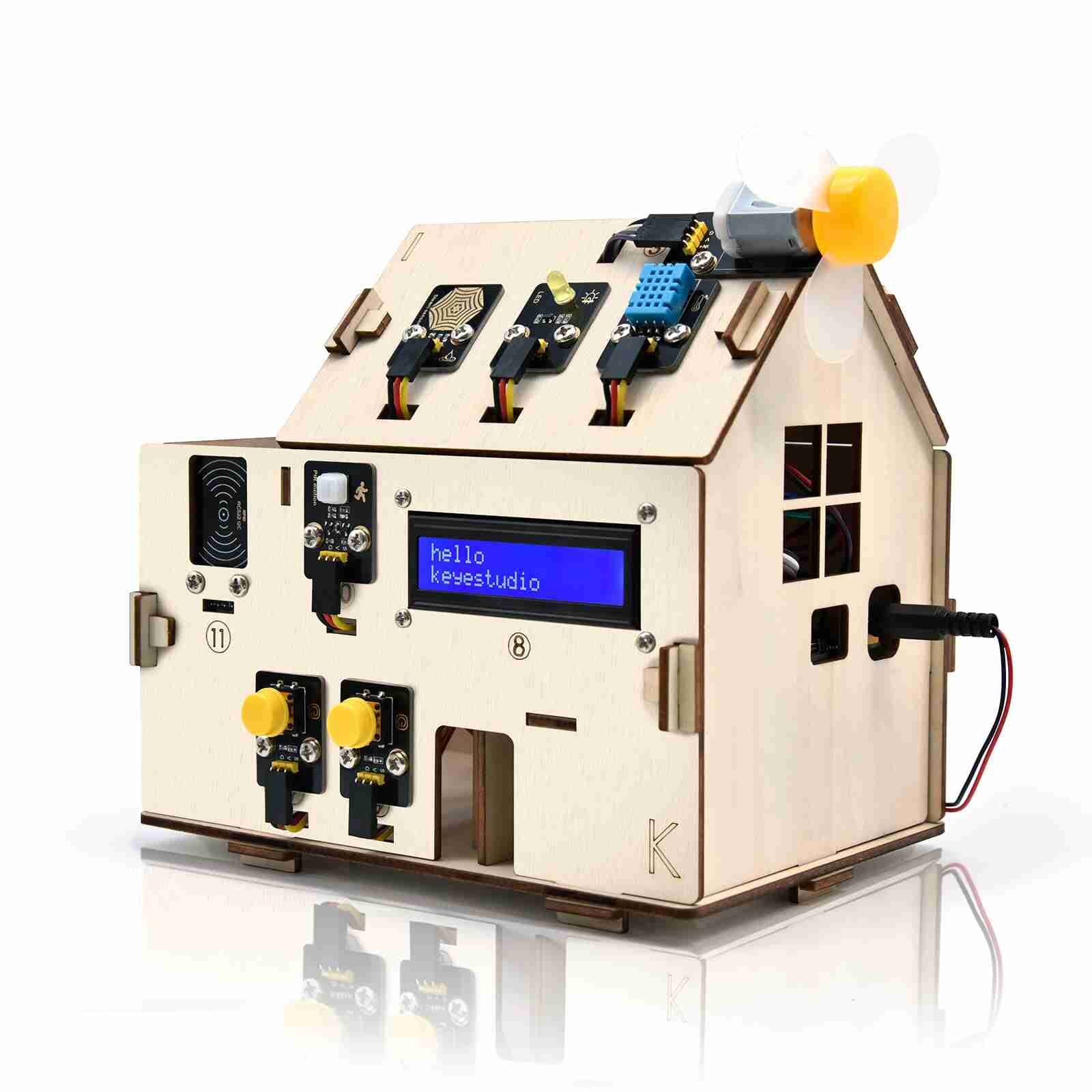
A few months ago I bought a Keyestudio Smart Home, assembled it and tried to program it using the Arduino IDE.
However I kept getting the following error when trying to upload a sketch to the board.
 avrdude: stk500_getsync() attempt 1 of 10: not in sync: resp=0x2e
 avrdude: stk500_getsync() attempt 2 of 10: not in sync: resp=0x2e
 avrdude: stk500_getsync() attempt 3 of 10: not in sync: resp=0x2e
Initially I thought it was an issue with the QinHeng Electronics CH340 serial converter driver software.
After exchanging a few emails with keyestudio support however I was pointed out that the board type of my smart home version was not “Arduino Uno”.
The box of the control board says “Keyestudio Control Board for ESP-32” and I had to install version 3.1.3 of the esp32 board software for being able to program the board.
I.e. the Keyestudio IoT Smart Home Kit for ESP32 is not to be confused with the Keyestudio Smart Home Kit for Arduino.
The documentation for the Keyestudio smart home using ESP-32 is here.
Also the correct version of the smart home sketches are here.
Finally you can find many sample projects in the keyestudio blog.
Note that in some cases you have to adapt the io pin numbers using the smart home documentation.
Many thanks to Keyestudio support for helping me to get it working.
I want to simulate an orbiting spacecraft using the Jolt Physics engine (see sfsim homepage for details).
The Jolt Physics engine solves difficult problems such as gyroscopic forces, collision detection with linear casting, and special solutions for wheeled vehicles with suspension.
The integration method of the Jolt Physics engine is the semi-implicit Euler method.
The following formula shows how speed v and position x are integrated for each time step:
\[
\begin{align*}
\mathbf{v}_{n+1} &= \mathbf{v}_n + \Delta t \, \mathbf{a}_n\\
\mathbf{x}_{n+1} &= \mathbf{x}_n + \Delta t \, \mathbf{v}_{n+1}
\end{align*}
\]
The orbital radius R was set to the Earth radius of 6378 km plus 408 km (the height of the ISS).
The Earth mass was assumed to be 5.9722e+24 kg.
For increased accuracy, the Jolt Physics library was compiled with the option -DDOUBLE_PRECISION=ON.
A full orbit was simulated using different values for the time step.
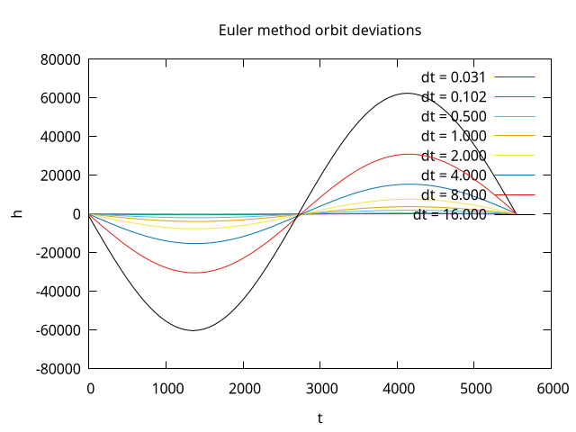
The following plot shows the height deviation from the initial orbital height over time.
When examining the data one can see that the integration method returns close to the initial after one orbit.
The orbital error of the Euler integration method looks like a sine wave.
Even for a small timestep of dt = 0.031 s, the maximum orbit deviation is 123.8 m.
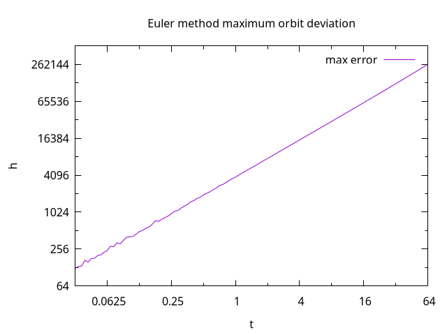
The following plot shows that for increasing time steps, the maximum error grows linearly.
For time lapse simulation with a time step of 16 seconds, the errors will exceed 50 km.
A possible solution is to use Runge Kutta 4th order integration instead of symplectic Euler.
The 4th order Runge Kutta method can be implemented using a state vector consisting of position and speed:
The Jolt Physics library allows to apply impulses to the spacecraft.
The idea is to use Runge Kutta 4th order integration to get an accurate estimate of the speed and position of the spacecraft after the next time step.
One can apply an impulse before running an Euler step so that the position after the Euler step matches the Runge Kutta estimate.
A second impulse then is used after the Euler time step to also make the speed match the Runge Kutta estimate.
Given the initial state (x(n), v(n)) and the desired next state (x(n+1), v(n+1)) (obtained from Runge Kutta) the formulas for the two impulses are as follows:
\[
\begin{align*}
\Delta\mathbf{i}_{n,0} &= m \, \Delta\mathbf{v}_{n,0} = \cfrac{m}{\Delta t}\,(\mathbf{x}_{n+1} - \mathbf{x}_n - \Delta t\,\mathbf{v}_n)\\
\Delta\mathbf{i}_{n,1} &= m \, \Delta\mathbf{v}_{n,1} = m \, (\mathbf{v}_{n+1} - \mathbf{v}_n - \Delta\mathbf{v}_{n,0})
\end{align*}
\]
The following code shows the implementation of the matching scheme using two speed changes in Clojure:
(defnmatching-scheme"Use two custom acceleration values to make semi-implicit Euler result match a ground truth after the integration step"[y0dty1scalesubtract](let[delta-speed0(scale(/1.0^doubledt)(subtract(subtract(:positiony1)(:positiony0))(scaledt(:speedy0))))delta-speed1(subtract(subtract(:speedy1)(:speedy0))delta-speed0)][delta-speed0delta-speed1]))
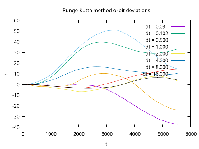
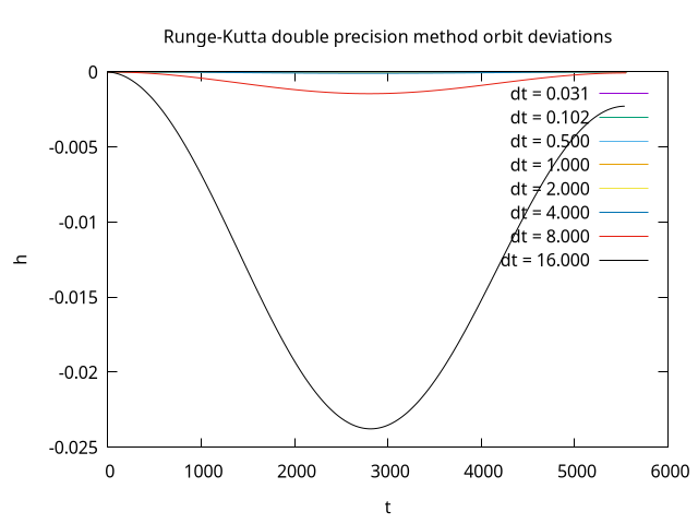
The following plot shows the height deviations observed when using Runge Kutta integration.
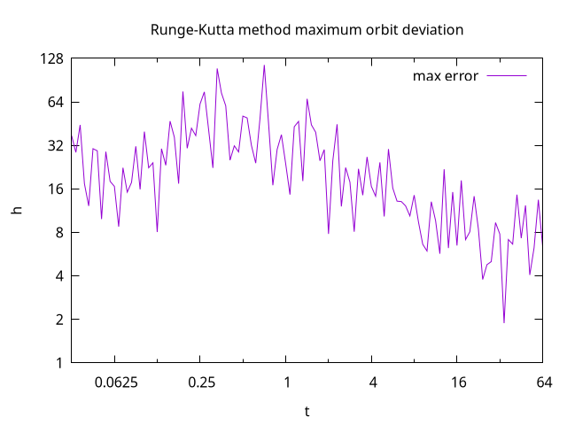
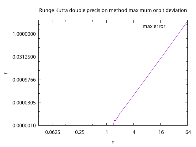
The following plot of maximum deviation shows that the errors are much smaller.
Although the accuracy of the Runge Kutta matching scheme is higher, a loss of 40 m of height per orbit is undesirable.
Inspecting the Jolt Physics source code reveals that the double-precision setting affects position vectors but is not applied to speed and impulse vectors.
To test whether double precision speed and impulse vectors would increase the accuracy, a test implementation of the semi-implicit Euler method with Runge Kutta matching scheme was used.
The following plot shows that the orbit deviations are now much smaller.
The updated plot of maximum deviation shows that using double precision the error for one orbit is below 1 meter for time steps up to 40 seconds.
I am currently looking into building a modified Jolt Physics version which uses double precision for speed and impulse vectors.
I hope that I will get the Runge Kutta 4th order matching scheme to work so that I get an integrated solution for numerically accurate orbits as well as collision and vehicle simulation.
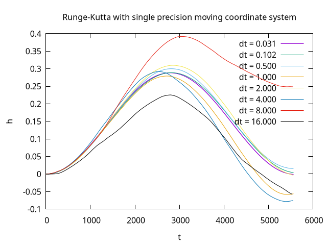
I have managed to get a prototype working using the moving coordinate system approach.
One can perform the Runge Kutta integration using double precision coordinates and speed vectors with the Earth at the centre of the coordinate system.
The Jolt Physics integration then happens in a coordinate system which is at the initial position and moving with the initial speed of the spaceship.
The first impulse of the matching scheme is applied and then the semi-implicit Euler integration step is performed using Jolt Physics with single precision speed vectors and impulses.
Then the second impulse is applied.
Finally the position and speed of the double precision moving coordinate system are incremented using the position and speed value of the Jolt Physics body.
The position and speed of the Jolt Physics body are then reset to zero and the next iteration begins.
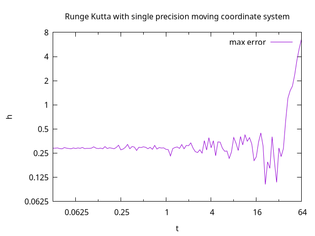
The following plot shows the height deviations observed using this approach:
The maximum errors for different time steps are shown in the following plot: