Orbits with Jolt Physics

I want to simulate an orbiting spacecraft using the Jolt Physics engine (see sfsim homepage for details). The Jolt Physics engine solves difficult problems such as gyroscopic forces, collision detection with linear casting, and special solutions for wheeled vehicles with suspension.

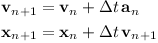
The integration method of the Jolt Physics engine is the semi-implicit Euler method. The following formula shows how speed v and position x are integrated for each time step:

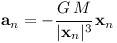
The gravitational acceleration by a planet is given by:

To test orbiting, one can set the initial conditions of the spacecraft to a perfect circular orbit:

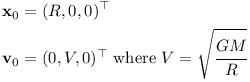
The orbital radius R was set to the Earth radius of 6378 km plus 408 km (the height of the ISS). The Earth mass was assumed to be 5.9722e+24 kg. For increased accuracy, the Jolt Physics library was compiled with the option -DDOUBLE_PRECISION=ON.

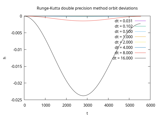
A full orbit was simulated using different values for the time step. The following plot shows the height deviation from the initial orbital height over time.

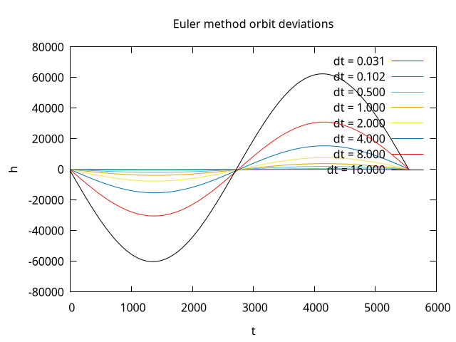
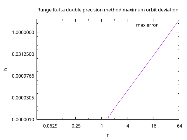
When examining the data one can see that the integration method returns close to the initial after one orbit. The orbital error of the Euler integration method looks like a sine wave. Even for a small timestep of dt = 0.031 s, the maximum orbit deviation is 123.8 m. The following plot shows that for increasing time steps, the maximum error grows linearly.

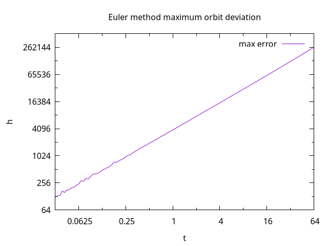
For time lapse simulation with a time step of 16 seconds, the errors will exceed 50 km.

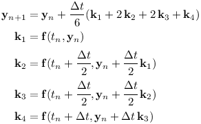
A possible solution is to use Runge Kutta 4th order integration instead of symplectic Euler. The 4th order Runge Kutta method can be implemented using a state vector consisting of position and speed:

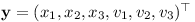
The derivative of the state vector consists of speed and gravitational acceleration:

The Runge Kutta 4th order integration method is as follows:

The Runge Kutta method can be implemented in Clojure as follows:

(defn runge-kutta
  "Runge-Kutta integration method"
  {:malli/schema [:=> [:cat :some :double [:=> [:cat :some :double] :some] add-schema scale-schema] :some]}
  [y0 dt dy + *]
  (let [dt2 (/ ^double dt 2.0)
        k1  (dy y0                0.0)
        k2  (dy (+ y0 (* dt2 k1)) dt2)
        k3  (dy (+ y0 (* dt2 k2)) dt2)
        k4  (dy (+ y0 (* dt  k3)) dt)]
    (+ y0 (* (/ ^double dt 6.0) (reduce + [k1 (* 2.0 k2) (* 2.0 k3) k4])))))

The following code can be used to test the implementation:

(def add (fn [x y] (+ x y)))
(def scale (fn [s x] (* s x)))

(facts "Runge-Kutta integration method"
       (runge-kutta 42.0 1.0 (fn [_y _dt] 0.0) add scale) => 42.0
       (runge-kutta 42.0 1.0 (fn [_y _dt] 5.0) add scale) => 47.0
       (runge-kutta 42.0 2.0 (fn [_y _dt] 5.0) add scale) => 52.0
       (runge-kutta 42.0 1.0 (fn [_y dt] (* 2.0 dt)) add scale) => 43.0
       (runge-kutta 42.0 2.0 (fn [_y dt] (* 2.0 dt)) add scale) => 46.0
       (runge-kutta 42.0 1.0 (fn [_y dt] (* 3.0 dt dt)) add scale) => 43.0
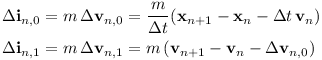
       (runge-kutta 1.0 1.0 (fn [y _dt] y) add scale) => (roughly (exp 1) 1e-2))

The Jolt Physics library allows to apply impulses to the spacecraft. The idea is to use Runge Kutta 4th order integration to get an accurate estimate of the speed and position of the spacecraft after the next time step. One can apply an impulse before running an Euler step so that the position after the Euler step matches the Runge Kutta estimate. A second impulse then is used after the Euler time step to also make the speed match the Runge Kutta estimate. Given the initial state (x(n), v(n)) and the desired next state (x(n+1), v(n+1)) (obtained from Runge Kutta) the formulas for the two impulses are as follows:

The following code shows the implementation of the matching scheme using two speed changes in Clojure:

(defn matching-scheme
  "Use two custom acceleration values to make semi-implicit Euler result match a ground truth after the integration step"
  [y0 dt y1 scale subtract]
  (let [delta-speed0 (scale (/ 1.0 ^double dt) (subtract (subtract (:position y1) (:position y0)) (scale dt (:speed y0))))
        delta-speed1 (subtract (subtract (:speed y1) (:speed y0)) delta-speed0)]
    [delta-speed0 delta-speed1]))

The following plot shows the height deviations observed when using Runge Kutta integration.

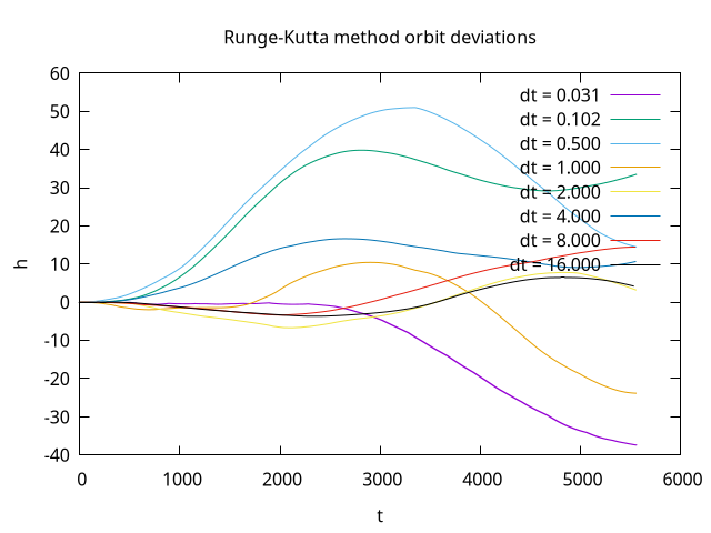
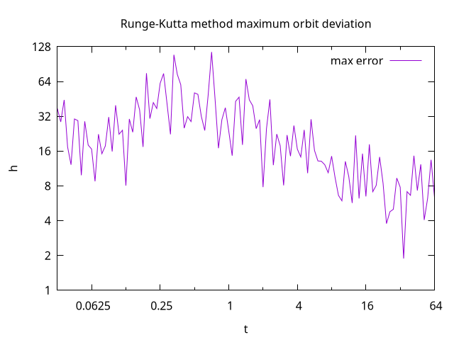
The following plot of maximum deviation shows that the errors are much smaller.

Although the accuracy of the Runge Kutta matching scheme is higher, a loss of 40 m of height per orbit is undesirable. Inspecting the Jolt Physics source code reveals that the double-precision setting affects position vectors but is not applied to speed and impulse vectors. To test whether double precision speed and impulse vectors would increase the accuracy, a test implementation of the semi-implicit Euler method with Runge Kutta matching scheme was used. The following plot shows that the orbit deviations are now much smaller.

The updated plot of maximum deviation shows that using double precision the error for one orbit is below 1 meter for time steps up to 40 seconds.

I am currently looking into building a modified Jolt Physics version which uses double precision for speed and impulse vectors. I hope that I will get the Runge Kutta 4th order matching scheme to work so that I get an integrated solution for numerically accurate orbits as well as collision and vehicle simulation.

Update:

Jorrit Rouwé has informed me that he currently does not want to add support for double precision speed values. He also has more detailed information about using Jolt Physics for space simulation on his website.

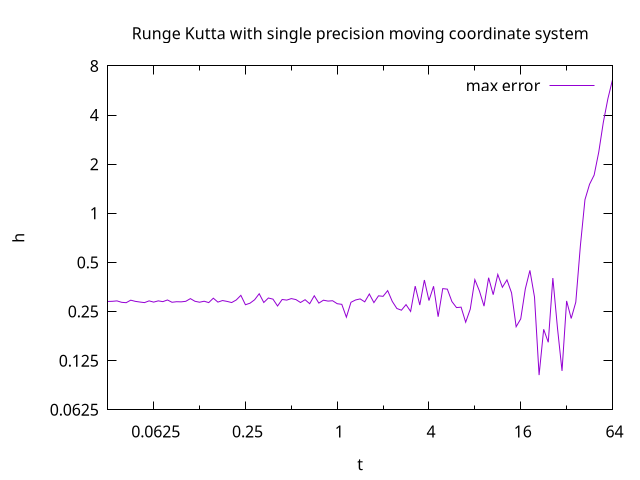
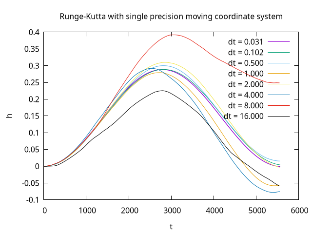
I have managed to get a prototype working using the moving coordinate system approach. One can perform the Runge Kutta integration using double precision coordinates and speed vectors with the Earth at the centre of the coordinate system. The Jolt Physics integration then happens in a coordinate system which is at the initial position and moving with the initial speed of the spaceship. The first impulse of the matching scheme is applied and then the semi-implicit Euler integration step is performed using Jolt Physics with single precision speed vectors and impulses. Then the second impulse is applied. Finally the position and speed of the double precision moving coordinate system are incremented using the position and speed value of the Jolt Physics body. The position and speed of the Jolt Physics body are then reset to zero and the next iteration begins.

The following plot shows the height deviations observed using this approach:

The maximum errors for different time steps are shown in the following plot: