Minimal OpenGL example in Clojure

Update:: I wrote a new article about using LWJGL 3 with Clojure.

Two years ago I published a minimal OpenGL example in C. Recently I got renewed interest in the Clojure programming language (if you want to learn Clojure, I can recommend the book Clojure in Action by the way). I hope to do some game development in Clojure. Initially I tried JOGL (Java Bindings for OpenGL), but then I switched to LWJGL version 2 (Lightweight Java Game Library). There is a Debian package for LWJGL version 2 and there is extensive documentation on the LWJGL Wiki. 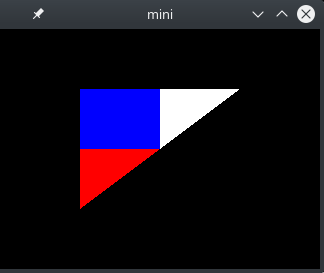Using this library, I have translated my earlier example to Clojure. See code below:

(ns raw-opengl
  (:import [org.lwjgl BufferUtils]
           [org.lwjgl.opengl Display DisplayMode GL11 GL12 GL13 GL15 GL20 GL30]))

(def vertex-source "#version 130
in mediump vec3 point;
in mediump vec2 texcoord;
out mediump vec2 UV;
void main()
{
  gl_Position = vec4(point, 1);
  UV = texcoord;
}")

(def fragment-source "#version 130
in mediump vec2 UV;
out mediump vec3 fragColor;
uniform sampler2D tex;
void main()
{
  fragColor = texture(tex, UV).rgb;
}")

(def vertices
  (float-array [ 0.5  0.5 0.0 1.0 1.0
                -0.5  0.5 0.0 0.0 1.0
                -0.5 -0.5 0.0 0.0 0.0]))

(def indices
  (int-array [0 1 2]))

(def pixels
  (float-array [0.0 0.0 1.0
                0.0 1.0 0.0
                1.0 0.0 0.0
                1.0 1.0 1.0]))

(defn make-shader [source shader-type]
  (let [shader (GL20/glCreateShader shader-type)]
    (GL20/glShaderSource shader source)
    (GL20/glCompileShader shader)
    (if (zero? (GL20/glGetShaderi shader GL20/GL_COMPILE_STATUS))
      (throw (Exception. (GL20/glGetShaderInfoLog shader 1024))))
    shader))

(defn make-program [vertex-shader fragment-shader]
  (let [program (GL20/glCreateProgram)]
    (GL20/glAttachShader program vertex-shader)
    (GL20/glAttachShader program fragment-shader)
    (GL20/glLinkProgram program)
    (if (zero? (GL20/glGetProgrami program GL20/GL_LINK_STATUS))
      (throw (Exception. (GL20/glGetProgramInfoLog program 1024))))
    program))

(defmacro def-make-buffer [method create-buffer]
  `(defn ~method [data#]
     (let [buffer# (~create-buffer (count data#))]
       (.put buffer# data#)
       (.flip buffer#)
       buffer#)))

(def-make-buffer make-float-buffer BufferUtils/createFloatBuffer)
(def-make-buffer make-int-buffer BufferUtils/createIntBuffer)

(Display/setTitle "mini")
(Display/setDisplayMode (DisplayMode. 320 240))
(Display/create)

(def vertex-shader (make-shader vertex-source GL20/GL_VERTEX_SHADER))
(def fragment-shader (make-shader fragment-source GL20/GL_FRAGMENT_SHADER))
(def program (make-program vertex-shader fragment-shader))

(def vao (GL30/glGenVertexArrays))
(GL30/glBindVertexArray vao)

(def vbo (GL15/glGenBuffers))
(GL15/glBindBuffer GL15/GL_ARRAY_BUFFER vbo)
(def vertices-buffer (make-float-buffer vertices))
(GL15/glBufferData GL15/GL_ARRAY_BUFFER vertices-buffer GL15/GL_STATIC_DRAW)

(def idx (GL15/glGenBuffers))
(GL15/glBindBuffer GL15/GL_ELEMENT_ARRAY_BUFFER idx)
(def indices-buffer (make-int-buffer indices))
(GL15/glBufferData GL15/GL_ELEMENT_ARRAY_BUFFER indices-buffer GL15/GL_STATIC_DRAW)

(GL20/glVertexAttribPointer (GL20/glGetAttribLocation program "point"   ) 3 GL11/GL_FLOAT false (* 5 Float/BYTES) (* 0 Float/BYTES))
(GL20/glVertexAttribPointer (GL20/glGetAttribLocation program "texcoord") 2 GL11/GL_FLOAT false (* 5 Float/BYTES) (* 3 Float/BYTES))
(GL20/glEnableVertexAttribArray 0)
(GL20/glEnableVertexAttribArray 1)

(GL20/glUseProgram program)

(def tex (GL11/glGenTextures))
(GL13/glActiveTexture GL13/GL_TEXTURE0)
(GL11/glBindTexture GL11/GL_TEXTURE_2D tex)
(GL20/glUniform1i (GL20/glGetUniformLocation program "tex") 0)
(def pixel-buffer (make-float-buffer pixels))
(GL11/glTexImage2D GL11/GL_TEXTURE_2D 0 GL11/GL_RGB 2 2 0 GL12/GL_BGR GL11/GL_FLOAT pixel-buffer)
(GL11/glTexParameteri GL11/GL_TEXTURE_2D GL11/GL_TEXTURE_WRAP_S GL11/GL_REPEAT)
(GL11/glTexParameteri GL11/GL_TEXTURE_2D GL11/GL_TEXTURE_MIN_FILTER GL11/GL_NEAREST)
(GL11/glTexParameteri GL11/GL_TEXTURE_2D GL11/GL_TEXTURE_MAG_FILTER GL11/GL_NEAREST)
(GL30/glGenerateMipmap GL11/GL_TEXTURE_2D)

(GL11/glEnable GL11/GL_DEPTH_TEST)

(while (not (Display/isCloseRequested))
  (GL11/glClearColor 0.0 0.0 0.0 0.0)
  (GL11/glClear (bit-or GL11/GL_COLOR_BUFFER_BIT GL11/GL_DEPTH_BUFFER_BIT))
  (GL11/glDrawElements GL11/GL_TRIANGLES 3 GL11/GL_UNSIGNED_INT 0)
  (Display/update)
  (Thread/sleep 40))

(GL20/glDisableVertexAttribArray 1)
(GL20/glDisableVertexAttribArray 0)

(GL11/glBindTexture GL11/GL_TEXTURE_2D 0)
(GL11/glDeleteTextures tex)

(GL15/glBindBuffer GL15/GL_ELEMENT_ARRAY_BUFFER 0)
(GL15/glDeleteBuffers idx)

(GL15/glBindBuffer GL15/GL_ARRAY_BUFFER 0)
(GL15/glDeleteBuffers vbo)

(GL30/glBindVertexArray 0)
(GL30/glDeleteVertexArrays vao)

(GL20/glDetachShader program vertex-shader)
(GL20/glDetachShader program fragment-shader)
(GL20/glDeleteProgram program)
(GL20/glDeleteShader vertex-shader)
(GL20/glDeleteShader fragment-shader)

(Display/destroy)

You can run the code as follows:

sudo apt-get install liblwjgl-java clojure
wget https://www.wedesoft.de/downloads/raw-opengl.clj
clojure -cp /usr/share/java/lwjgl.jar raw-opengl.clj

Any feedback, comments, and suggestions are welcome.

Enjoy!

Update:

If you are using Clojure 1.11 or later, you need to use a deps.edn file or specify the dependency on the command line like this:

clj -Sdeps '{:deps {lwglj/lwglj {:local/root "/usr/share/java/lwjgl.jar"}}}' -M raw-opengl.clj

The MealMaster file format

The MealMaster file format (*.MMF or *.MM file) is a popular file format for sharing recipes. MealMaster is the file format introduced by the MealMaster software developed by Episoft Systems.

The website of Episoft Systems, which provided the original MealMaster software for DOS, is not online any more. Fortunately a copy of the website is still available on the Internet Archive.

If you are looking for a MealMaster compatible recipe management software, please checkout my project AnyMeal!

One-column format

Below follows an example of the one-column MealMaster format (the ingredients are listed in a single column).

MMMMM----------------Meal-Master recipe exported by AnyMeal-----------------
     Title: Fruit-Meringue-Pie
Categories: pastries,cakes
  Servings: 1 pie

MMMMM----------------------------sponge mixture-----------------------------
    150 g  soft butter
    150 g  sugar
      3    eggs
    150 g  flour
      1 ts baking powder
MMMMM-------------------------------meringue--------------------------------
      4    egg white
    150 g  sugar
     50 g  almond leaves
MMMMM-------------------------------filling---------------------------------
    370 g  sour cherries;dripped off (
           -1 glass)
  1 1/2 tb cornflour
    1/4 l  cherry juice
    250 g  cream
      1 tb sugar
      1 pk stabiliser

Butter spring form with butter paper. Preheat oven to 200°.

MMMMM----------------------------sponge mixture-----------------------------
Stir butter, sugar and eggs until foamy, mix flour and baking powder and stir
in. Fill dough in in two spring forms and smooth down. Pre-bake for 15
minutes.

MMMMM-------------------------------meringue--------------------------------
Beat egg white until stiff and let sugar trickle in spoon by spoon. Beat
until stiff. Spread meringue base on pre-backed flan bases. Scatter almond
leaves over them. Bake for further 10-15 minutes. Let flan bases cool down on
a grid.

MMMMM-------------------------------filling---------------------------------
For the filling mix cornflour with some cherry juice. Bring remaining juice
to boiling point, stir in cornflour and boil up. Mix in sour cherries, let
cool down a bit and spread over one flan base.

Beat cream with sugar and stabiliser until stiff, spread over filling.
Cut second flan base in 12 pieces and reassemble on top of the filling. Let
cool down well.

MMMMM

The recipe header begins with MMMMM or —–. The header also has to contain the word “Meal-Master”. The recipe content then starts with a title of up to 60 characters. Then a list of categories follows. Each category can have up to 11 characters. Then servings amount and unit are specified.

In this recipe there are three ingredient sections. An ingredient section starts with MMMMM or —–. Ingredient amounts are specified in column 1 to 7. Column 9 and 10 specify the unit token. Starting from column 12 ingredient text of up to 28 characters follows. If the ingredient text is longer than 28 characters, it is broken up using ingredient continuation lines. Ingredient continuation lines begin with a “-“ in column 12.

Finally the instruction text follows. The instruction text also can be split up into multiple sections starting with MMMMM or —–. The recipe ends with MMMMM.

Two-column format

Here is an example of the two-column format. The ingredients are listed in two columns.

---------- Recipe via Meal-Master (tm) v8.01

      Title: Cannoli
 Categories: Italian, Desserts
      Yield: 16 servings

----------------------------------FILLING----------------------------------
  1 1/2 c  Whole-milk ricotta cheese;      1 1/2 c  Milk chocolate;
           - well drained                           - coarsely chopped
      3 tb Sugar                             1/4 c  Pistachio nuts;
  1 1/2 ts Cinnamon                                 - coarsely chopped

-----------------------------------DOUGH-----------------------------------
      1 c  All-purpose flour                        - or dry white wine
      1 tb Sugar                               2 c  Vegetable oil
      1 tb Butter or lard                           Colored sprinkles
      4 tb To 5 Tbl sweet Marsala wine

  In a bowl, combine all the filling ingredients and mix well. Refreigerate,
  covered, until ready to fill the cannoli shells.

  To make the dough, place the flour in a bowl or food processor. Add the
  butter or lard and sugar and mix with a fork, or pulse, until the mixture
  resembles coarse meal. Slowly add the 1/4 cup of wine and shape the mixture
  into a ball; add a little more wine if the dough appears too dry. It should
  be soft but not sticky. Knead the dough on a floured surface until smooth,
  about 10 minutes.  Wrap the dough and refrigerate for 45 minutes.

  Place the chilled dough on a floured work surface. Divide the dough in
  half.  Work with 1 piece of dough at a time; keep the remaining dough
  refrigerated. Roll the dough out to a very thin long rectangle about 14
  inches long and 3 inches wide, either by hand or using a pasta machine set
  to the finest setting.  Cut the dough into 3-inch squares. Place a cannoli
  form diagnoally across 1 square. Roll the dough up around the form so the
  points meet in the center.  Seal the points with a little water. Continue
  making cylinders until all the dough is used.

  In an electric skillet, heat the vegetable oil to 375F. Fry the cannoli 3
  or 4 at a time, turning them as they brown and blister, until golden brown
  on all sides. Drain them on brown paper. When they are cool enough to
  handle, carefully slide the cannoli off the forms.

  To serve, use a long iced tea spoon or a pastry bag without a tip to fill
  the cannoli with the ricotta cheese mixture. Dip the ends into colored
  sprinkles, arrange them on a tray, and sprinkle confectioner's sugar over
  the tops.  Serve at once.

  NOTE:  If you prefer, you can fry the cannoli in a deep fryer. Be sure to
  fill the cannoli just before serving - any sooner will make the shells
  soggy.

  This recipe from CIAO ITALIA by Mary Ann Esposito

-----

Here “Yield” is used instead of “Servings”. Note that the order of ingredients in each section is column major. In this example the second ingredient section has a second column starting with an ingredient continuation line. I.e. it is continuing the last ingredient of the first column.

This example also shows instruction text being indented by two spaces. Empty lines are used to create paragraphs.

The recipe ends with —–.

Not shown in these examples is to use an instruction line beginning with a “:” to force a line break.

Units

The following table shows the meaning of each of the unit tokens:

See Wikipedia page on approximate measures for more details.

Grammar

Here is an ABNF grammar of the MealMaster file format:

Mealmaster   = recipe Mealmaster
               / *( VCHAR / SP ) eol Mealmaster
               /
recipe       = header title categories servings ingredients instructions footer
header       = separator *( VCHAR / SP ) "Meal-Master" *( VCHAR / SP ) eol
title        = '     Title: ' 0*60( VCHAR / SP ) eol
categories   = 'Categories: ' categlist eol
categlist    = 1*11( VCHAR / SP ) ["," categlist]
servings     = '  Servings: ' 1*4( DIGIT ) [ SP [ 1*10( VCHAR / SP ) ] ] eol
ingredients  = onecolumn
               / twocolumn
onecolumn    = section onecolumn
               / ingredone eol onecolumn
               / *( SP ) eol onecolumn
               /
twocolumn    = section twocolumn
               / ingredtwo SP ingredone eol twocolumn
               / ingredone eol [ *( eol ) section twocolumn ]
               /
ingredone    = amount SP unit SP 1*28( VCHAR / SP )
ingredtwo    = amount SP unit SP 28( VCHAR / SP )
amount       = 7( SP / DIGIT / "." / "/" )
unit         = 'x ' / 'sm' / 'md' / 'lg' / 'cn' / 'pk' / 'pn' / 'dr' / 'ds'
               / 'ct' / 'bn' / 'sl' / 'ea' / 't ' / 'ts' / 'T ' / 'tb' / 'fl'
               / 'c ' / 'pt' / 'qt' / 'ga' / 'oz' / 'lb' / 'ml' / 'cb' / 'cl'
               / 'dl' / 'l ' / 'mg' / 'cg' / 'dg' / 'g ' / 'kg' / '  '
instructions = 0*255( VCHAR ) eol instructions
               / section instructions
               /
section      = separator *( VCHAR / SP ) eol
footer       = separator eol
separator    = 'MMMMM'
               / '-----'
eol          = [ CR ] LF

The grammar uses several rules from the ABNF standard:

• / is used to specify alternative rules.
• VCHAR stands for any printable character (except whitespace)
• DIGIT is a digit (one of 0,1,2,3,…,9).
• SP is the space character.
• CR means carriage return (0x0D).
• LF is the line-feed character (0x0A).
• *( VCHAR / SP ) means any number of printable and space characters or no characters at all.
• 1*4( DIGIT ) is used to specify one to four digits.
• [ CR ] is an optional carriage return character.
• 5( ‘M’ ) is exactly 5 capital “M”-characters.

Conclusion

The MealMaster file format is quite difficult to parse. Also there are a few problems with the file format:

• It is not possible to protect a comma in a category-name from interpretation as a separator.
• To prevent an occurrence of —–, : or MMMMM in the instructions-text from being interpreted as a special token, some recipe applications prepend all instruction lines with two space characters, which need to be ignored during import.
• The original Mealmaster software will refuse to import recipes exceeding a certain size. Also overlong titles, categories, and servings will be cropped.
• There are many recipes with ingredient-text longer than 28 characters. Overlong ingredient lines are making it more difficult to distinguish between the one- and two-column format.
• The ending of the ingredient section is not defined properly.
• Some recipe applications are relying on an empty line separating the ingredients from the instructions. On the other hand the original Mealmaster application allows empty lines within the ingredient-section.
• There are recipe applications exporting MealMaster files containing categories with more than 11 characters.

I hope this description will be useful to you if you are trying to parse MealMaster recipes. Please let me know any feedback in the comment section below.

New revamped version of the AnyMeal recipe management software

More than 15 years ago after leaving university I developed a GNU/Linux software called AnyMeal for managing a large amount of recipes. The software was based on the MealMaster file format which is a popular file format for sharing recipes.

The website of Episoft Systems, which provided the original MealMaster software for DOS, is not online any more. Fortunately a copy of the website is still available on the Internet Archive.

The AnyMeal software used the recode library to convert recipe text files to the UTF-8 encoding. A fast Flex parser then converted the MealMaster recipes to XML. An XSLT script was used to generate SQL commands for inserting the recipe into a MySQL database. For setting up the database and user account, the software had a step-by-step wizard. The KDE password manager was used to store the user credentials.

The recipe search was performed using a complicated search dialog with multiple tabs. The graphical user interface used multiple windows to display recipes and lists of search results. A recipe editor was implemented for modifying existing recipes or adding new ones.

However life happened and eventually I stopped maintaining the software. The software was developed using Qt3 and when Qt4 came out, there were breaking changes with list views and the software didn’t work on new systems any more.

Now many years later it still looks like there is a space for a fast recipe management software which can handle a large amount of MealMaster recipes. So I decided to use my past experience and do a rewrite of the old software.

This time I used the Qt5 framework to implement the graphical user interface. Instead of the old list view items, Qt5 now uses an item model and a list view widget to view the model. Also Qt5 provides cross-platform support for printing which is a great feature for a recipe management software. Like that it is not necessary to have a computer in the kitchen any more ;)

Instead of MySQL, I used the SQLite3 embedded database. This greatly simplified the software because SQLite3 does not require the setup of user accounts and databases. Also the user does not have to run a database server in the background. Furthermore without user credentials there is no need for interfacing with the KDE password manager any more.

For the internal representation of recipes I decided to use a more conservative approach. For representing recipes I used a C++ class instead of XML data. Like that it is not necessary to depend on the Xalan XSLT processor and Xerces-C XML library any more.

I also changed the order of UTF-8 conversion and parsing of recipes. Now the recipes are first parsed with an Flex MealMaster parser and stored as C++ objects. The strings of the C++ object then get converted to UTF-8 using the recode library. Like that it is not necessary for the Flex parser to be UTF-8 aware any more thus simplifying the implementation.

The search was also simplified. A search can be performed on title, category, or ingredient. It is possible to narrow down the search result by using several searches one by one. I.e. it is not necessary any more to implement a complicated search dialog which builds a complex search query.

Back then I used CVS for version control. This time the version control was done using Git. AnyMeal is still hosted on SourceForge however the source repository is now on Github, Gitlab, and BitBucket (after all Git is a distributed version control system!). The main project page is on Github (which displays the content of the gh-pages branch of the repository).

After simplifying the software architecture like that, it was possible to implement the software in less than 100 hours. Most of the work of the rewrite was implementing a simpler Flex parser and reimplementing the recipe editor. In contrast to back then, I implemented the internals of the application using test-driven development (TDD). I used Google Test which is Google’s C++ test framework. Also, unlike back then, now there is Travis CI which provides free automated testing for software libre.

Finally using MSYS and MinGW the software was also compiled for Microsoft Windows. The Nullsoft Scriptable Install System (NSIS) was used to create an installer.

I am planning to add a few more small features but I think the software is more or less ready to be used for cooking.

Let me know what you think in the comment section below.

Enjoy!

Update:

Article was submitted to Hacker News.

I also forgot to mention that I used Docker and debuild to create a package for Debian Sid.

Rigid body game physics 6

part 1 part 2 part 3 part 4 part 5 part 6

Update: See Getting started with the Jolt Physics Engine

A realistic simulation requires the estimation of friction forces.

Friction Forces

Colliding as well as resting contacts cause constraint impulses as well as friction impulses. So far we have only estimated the constraint impulses of colliding and resting contacts. Constraint impulses are in the direction of the contact’s normal vector. Friction impulses act tangential to the contact plane (orthogonal to the normal vector). The inequality constraint is J and b have two rows. The vectors t1 and t2 are chosen so that they are orthogonal to the normal vector n and orthogonal to each other. Friction forces try to reduce tangential velocities to zero. I.e. b is

The linear components of J are and the angular components of J are

As before λ is computed Here λ has two elements. λ1 and λ2 are scaled with the same positive factor if necessary so that the length of the 2D vector consisting of λ1 and λ2 is smaller than the normal impulse Pn multiplied with the friction constant μ. Basically the overall force vector needs to reside in the friction cone. In a similar fashion as for constraint impulses, friction impulses are subtracted, recomputed, and then added to the accumulated impulses P of the two objects, when iterating.

If you have made it this far, you know how to build a small physics engine!

Any feedback, comments, and suggestions are welcome.

Further reading

• K. Erleben: Stable, robust, and versatile multibody dynamics animation
• B. Mirtich: Impulse-based dynamics simulation of rigid body systems
• H. Eichner: Rigid Body Game Physics

Rigid body game physics 5

part 1 part 2 part 3 part 4 part 5 part 6

In order to handle collisions and resting contacts, it is necessary to determine contact points. One can achieve this using the separating plane algorithm (also see Baraff).

Separating Planes Algorithm

The separating plane algorithm only applies to convex polyhedra. However non-convex objects can in many cases be approximated by a union of convex polyhedra. A separating plane is a plane such that all points of the polyhedra A and B lie on opposite sides of the plane. If two polyhedra are not intersecting, a separating plane can either be defined using one of the faces of one of the polyhedra or be constructed from one edge of A and one edge of B.

The distance d of a point x from the plane P(p,n) defined by the point p and the normal vector n is:

1. In the case of using a face from polyhedron A, the point p is a corner of the face. The normal vector n is the normalized cross product of two edges of the face and pointing outward from the polyhedron. The point x of polyhedron B with the smallest distance d defines the distance of B to the face of A. If this distance is positive, the face of polyhedron A is a separating plane.

2. In the case of using two edges, the point p is the corner of an edge from polyhedron A. The normal vector n is the positive or negative normalized cross product of the two edge vectors. Again the point x of polyhedron B with the smallest distance d defines the distance of B to the face of A.

From all the planes, the one with the largest distance d is selected. If the distance is zero or negative, the two polyhedra are in contact. One can place a plane in the “middle” of the contact by moving it by half the distance d, i.e.

In the next step all points from A and B, which have a distance less than ε to the plane, are selected. Two vectors u and v orthogonal to the normal n and orthogonal to each other are determined. The points are projected onto the plane and represented using the vectors u and v: The convex hull of the each of the two polygons is determined. Then the intersection of the resulting two 2D polygons is computed. Finally the convex hull of the intersection is taken. The points are projected back into 3D space. These are the contact points used for simulating the colliding and resting contacts.